<?xml version="1.0" encoding="utf-8"?><feed xmlns="http://www.w3.org/2005/Atom" ><generator uri="https://jekyllrb.com/" version="3.10.0">Jekyll</generator><link href="https://dpm24800.github.io/feed.xml" rel="self" type="application/atom+xml" /><link href="https://dpm24800.github.io/" rel="alternate" type="text/html" /><updated>2026-04-02T02:33:32+00:00</updated><id>https://dpm24800.github.io/feed.xml</id><title type="html">🧭 The Path</title><subtitle>Welcome to my GitHub Pages site — a space where I document my learning journey in Data Science, Machine Learning, and AI. I share technical notes, tutorials, projects, and reflections on Dhamma and mindfulness, blending analytical curiosity with inner understanding.
</subtitle><author><name>Dipak Pulami Magar</name></author><entry><title type="html">Reflections</title><link href="https://dpm24800.github.io/dhamma/reflections/2026/04/01/reflections.html" rel="alternate" type="text/html" title="Reflections" /><published>2026-04-01T21:27:45+00:00</published><updated>2026-04-01T21:27:45+00:00</updated><id>https://dpm24800.github.io/dhamma/reflections/2026/04/01/reflections</id><content type="html" xml:base="https://dpm24800.github.io/dhamma/reflections/2026/04/01/reflections.html"><![CDATA[<h2 id="2026-04-02">2026-04-02</h2>
<ul>
  <li>It takes a little time to realize that – (these/those) things were not meant for me / were never meant for me. <a href="https://www.facebook.com/photo?fbid=122184393716757213&amp;set=a.122130586082757213">IMG</a></li>
  <li></li>
</ul>]]></content><author><name>Dipak Pulami Magar</name></author><category term="dhamma" /><category term="reflections" /><summary type="html"><![CDATA[2026-04-02 It takes a little time to realize that – (these/those) things were not meant for me / were never meant for me. IMG]]></summary></entry><entry><title type="html">Encoding vs Embedding</title><link href="https://dpm24800.github.io/deep-learning/nlp/2026/03/30/encoding-vs-embeddings.html" rel="alternate" type="text/html" title="Encoding vs Embedding" /><published>2026-03-30T23:15:00+00:00</published><updated>2026-03-30T23:15:00+00:00</updated><id>https://dpm24800.github.io/deep-learning/nlp/2026/03/30/encoding-vs-embeddings</id><content type="html" xml:base="https://dpm24800.github.io/deep-learning/nlp/2026/03/30/encoding-vs-embeddings.html"><![CDATA[<p>Let’s imagine you are teaching a computer to understand words like <strong>“cat”, “dog”, and “tiger.”</strong>
The problem is: computers don’t understand words — they only understand <strong>numbers</strong>.</p>

<p>So we need a way to <strong>turn words into numbers</strong>.</p>

<p>That’s where <strong>encoding</strong> and <strong>embedding</strong> come in.</p>

<h1 id="1-step-one-what-is-encoding">1. Step One: What is Encoding?</h1>

<p>Think of <strong>encoding</strong> as giving each word a number tag.</p>

<h3 id="example">Example:</h3>

<p>You have 3 animals:</p>

<ul>
  <li>cat</li>
  <li>dog</li>
  <li>tiger</li>
</ul>

<h3 id="method-1-label-encoding">Method 1: Label Encoding</h3>

<p>We assign numbers:</p>

<ul>
  <li>cat → 0</li>
  <li>dog → 1</li>
  <li>tiger → 2</li>
</ul>

<p>But here’s the problem:</p>

<ul>
  <li>The computer might think <strong>tiger (2) &gt; dog (1)</strong></li>
  <li>But animals don’t work like that!</li>
</ul>

<h3 id="method-2-one-hot-encoding">Method 2: One-Hot Encoding</h3>

<p>Instead, we use a special trick:</p>

<ul>
  <li>cat → <code class="language-plaintext highlighter-rouge">[1, 0, 0]</code></li>
  <li>dog → <code class="language-plaintext highlighter-rouge">[0, 1, 0]</code></li>
  <li>tiger → <code class="language-plaintext highlighter-rouge">[0, 0, 1]</code></li>
</ul>

<p>Now:</p>

<ul>
  <li>No number is “bigger” than another</li>
  <li>Everything is treated equally</li>
</ul>

<h3 id="but-there-is-still-a-big-problem">But there is still a big problem…</h3>

<p>Look at:</p>

<ul>
  <li>cat → <code class="language-plaintext highlighter-rouge">[1, 0, 0]</code></li>
  <li>tiger → <code class="language-plaintext highlighter-rouge">[0, 0, 1]</code></li>
</ul>

<p>To the computer, these are <strong>completely different</strong>.</p>

<p>But in real life:</p>

<ul>
  <li>cat and tiger are <strong>very similar</strong> (both are cats!)</li>
</ul>

<p>Encoding <strong>does NOT understand meaning</strong>.</p>

<h1 id="2-step-two-what-is-embedding">2. Step Two: What is Embedding?</h1>

<p>Now comes the smart idea.</p>

<p>Instead of assigning numbers manually, we let the computer <strong>learn the numbers by itself</strong>.</p>

<p>This is called <strong>embedding</strong>.</p>

<h2 id="imagine-a-map-of-words">Imagine a Map of Words</h2>

<p>Think of a 2D map like a game world:</p>

<ul>
  <li>“cat” is placed here</li>
  <li>“tiger” is placed nearby</li>
  <li>“car” is placed far away</li>
</ul>

<p>So:</p>

<ul>
  <li>Similar things are <strong>close together</strong></li>
  <li>Different things are <strong>far apart</strong></li>
</ul>

<h3 id="example-embeddings">Example Embeddings</h3>

<ul>
  <li>cat → <code class="language-plaintext highlighter-rouge">[0.2, 0.8]</code></li>
  <li>tiger → <code class="language-plaintext highlighter-rouge">[0.25, 0.75]</code></li>
  <li>car → <code class="language-plaintext highlighter-rouge">[0.9, 0.1]</code></li>
</ul>

<p>Now:</p>

<ul>
  <li>cat and tiger are <strong>close → similar</strong></li>
  <li>car is <strong>far → different</strong></li>
</ul>

<p>This is something encoding could never do.</p>

<h1 id="3-how-does-the-computer-learn-this">3. How Does the Computer Learn This?</h1>

<p>This is the magical part.</p>

<p>The computer learns embeddings by reading lots of sentences like:</p>

<ul>
  <li>“The cat drinks milk”</li>
  <li>“The tiger hunts in the jungle”</li>
</ul>

<p>It notices:</p>

<ul>
  <li>cat and tiger appear in <strong>similar contexts</strong></li>
  <li>so they must be <strong>related</strong></li>
</ul>

<p>And it slowly adjusts numbers to reflect that.</p>

<h1 id="4-simple-analogy">4. Simple Analogy</h1>

<h3 id="encoding-is-like">Encoding is like:</h3>

<p>Giving every student in a class a <strong>roll number</strong></p>

<ul>
  <li>Rahul → 1</li>
  <li>Sita → 2</li>
</ul>

<p>But roll numbers don’t tell you:</p>

<ul>
  <li>who is good at math</li>
  <li>who likes football</li>
</ul>

<h3 id="embedding-is-like">Embedding is like:</h3>

<p>Giving each student a <strong>profile based on personality</strong></p>

<ul>
  <li>Rahul → good at math, likes cricket</li>
  <li>Sita → likes art, good at music</li>
</ul>

<p>Now you can:</p>

<ul>
  <li>group similar students</li>
  <li>understand relationships</li>
</ul>

<h1 id="5-why-embeddings-are-powerful">5. Why Embeddings Are Powerful</h1>

<p>With embeddings, a computer can:</p>

<ul>
  <li>Understand <strong>similar words</strong></li>
  <li>
    <p>Do analogies:</p>

    <ul>
      <li>king − man + woman ≈ queen</li>
    </ul>
  </li>
  <li>
    <p>Improve tasks like:</p>

    <ul>
      <li>translation</li>
      <li>sentiment analysis</li>
      <li>chatbots</li>
    </ul>
  </li>
</ul>

<h1 id="6-key-differences">6. Key Differences</h1>

<table>
  <thead>
    <tr>
      <th>Encoding</th>
      <th>Embedding</th>
    </tr>
  </thead>
  <tbody>
    <tr>
      <td>Just assigns numbers</td>
      <td>Learns meaningful numbers</td>
    </tr>
    <tr>
      <td>No understanding</td>
      <td>Understands relationships</td>
    </tr>
    <tr>
      <td>Sparse (lots of zeros)</td>
      <td>Dense (compact info)</td>
    </tr>
    <tr>
      <td>Manual rules</td>
      <td>Learned automatically</td>
    </tr>
  </tbody>
</table>

<h1 id="7-in-deep-learning">7. In Deep Learning</h1>

<p>When you use:</p>

<div class="language-python highlighter-rouge"><div class="highlight"><pre class="highlight"><code><span class="n">Embedding</span><span class="p">(</span><span class="n">vocab_size</span><span class="p">,</span> <span class="n">vector_size</span><span class="p">)</span>
</code></pre></div></div>

<p>You are telling the model:</p>

<blockquote>
  <p>“Don’t just label words…
<strong>learn their meaning from data.</strong>”</p>
</blockquote>

<h1 id="8-final-intuition">8. Final Intuition</h1>

<ul>
  <li><strong>Encoding</strong> = “Here is a number for each word.”</li>
  <li><strong>Embedding</strong> = “Here is what this word <em>means</em> in numbers.”</li>
</ul>

<h1 id="9-one-line-summary">9. One-Line Summary</h1>

<blockquote>
  <p>Encoding helps the computer <strong>see words</strong>,
Embedding helps the computer <strong>understand words</strong>.</p>
</blockquote>]]></content><author><name>Dipak Pulami Magar</name></author><category term="deep-learning" /><category term="nlp" /><summary type="html"><![CDATA[Let’s imagine you are teaching a computer to understand words like “cat”, “dog”, and “tiger.” The problem is: computers don’t understand words — they only understand numbers.]]></summary></entry><entry><title type="html">Demystifying K-Means Clustering</title><link href="https://dpm24800.github.io/machine-learning/unsupervised/clustering/2026/03/17/k-means-clustering.html" rel="alternate" type="text/html" title="Demystifying K-Means Clustering" /><published>2026-03-17T10:15:00+00:00</published><updated>2026-03-17T10:15:00+00:00</updated><id>https://dpm24800.github.io/machine-learning/unsupervised/clustering/2026/03/17/k-means-clustering</id><content type="html" xml:base="https://dpm24800.github.io/machine-learning/unsupervised/clustering/2026/03/17/k-means-clustering.html"><![CDATA[<p>Welcome to a detailed exploration of K-Means Clustering, one of the most fundamental algorithms in data science. This blog post isn’t just a conceptual overview—it is a complete journey, starting from the basic definitions, walking through a mathematical example calculation step by step, showing how to implement it in Python, and finally, explaining how to measure success.</p>

<p>Whether you are a student, a beginner, or just need a solid refresh, this guide will make K-Means crystal clear.</p>

<hr />

<h2 id="1-introduction-to-clustering">1. Introduction to Clustering</h2>

<p>Before we dive into the algorithm, let’s establish the context: unsupervised machine learning.</p>

<h3 id="what-is-clustering">What is Clustering?</h3>

<p>At its heart, <strong>Clustering</strong> is about finding groups within data. It is the process of <strong>grouping similar data points together</strong> while keeping dissimilar points separated.</p>

<p>It is a type of <strong>unsupervised learning</strong>, which means the algorithm works on unlabeled data. We don’t have a “right answer” (a label like “cat” or “dog”); the algorithm must discover the structure, patterns, and relationships within the data on its own.</p>

<h3 id="applications-of-clustering">Applications of Clustering</h3>

<p>If you need to make sense of large amounts of diverse data without previous categories, clustering is your go-to tool. It is used in:</p>

<ul>
  <li><strong>Customer Segmentation:</strong> Businesses analyze purchasing behavior to group customers (e.g., “high spenders,” “occasional buyers”) for targeted marketing.</li>
  <li><strong>Image Compression:</strong> By grouping pixels with similar colors together and using the group center as a single color, images can be compressed significantly.</li>
  <li><strong>Anomaly Detection:</strong> By clustering standard patterns of data (like bank transactions or sensor readings), data points that fall far outside of any cluster can be identified as potential fraud or system errors.</li>
</ul>

<hr />

<h2 id="2-what-is-k-means">2. What is K-Means?</h2>

<h3 id="the-core-concept">The Core Concept</h3>

<p><strong>K-Means</strong> is a specific, popular <strong>partitioning-based clustering algorithm</strong>. Its objective is to divide a dataset into \(K\) distinct, non-overlapping subsets (clusters) based on the similarity of the data points.</p>

<h3 id="the-objective-function">The Objective Function</h3>

<p>The main goal of K-Means can be summarized as:</p>

<ol>
  <li><strong>Minimize Intra-cluster distance:</strong> Make points inside the same cluster as close (similar) as possible to each other. This is measured by how close points are to their cluster center (centroid).</li>
  <li><strong>Maximize Inter-cluster distance:</strong> Keep the clusters themselves as far away (dissimilar) as possible from each other.</li>
</ol>

<hr />

<h2 id="3-how-k-means-works-step-by-step">3. How K-Means Works (Step-by-Step)</h2>

<p>The beauty of K-Means lies in its simple, iterative process. Here is how it functions, step-by-step:</p>

<p>[Image: A diagram showing the iterative steps of K-Means Clustering]</p>

<h3 id="step-1-choose-k">Step 1: Choose K</h3>

<p>The first and most critical decision is deciding the number of clusters, \(K\). We will discuss how to choose this optimally later.</p>

<h3 id="step-2-initialize-centroids">Step 2: Initialize Centroids</h3>

<p>K-Means starts by placing \(K\) points into the feature space. These initial points are called <strong>centroids</strong> (the centers of the clusters).</p>

<ul>
  <li>They can be initialized <strong>randomly</strong> by picking \(K\) random data points from the dataset.</li>
  <li>Better methods exist, such as <strong>K-Means++</strong>, which initializes centroids far apart from each other, speeding up convergence and avoiding bad local optima.</li>
</ul>

<h3 id="step-3-assign-points">Step 3: Assign Points</h3>

<p>This is the optimization part. For every single data point in your entire dataset:</p>

<ol>
  <li>Calculate its distance to all \(K\) centroids.</li>
  <li>Assign the point to the cluster of the <strong>nearest</strong> centroid.</li>
</ol>

<p>A point is assigned to Cluster \(j\) if the distance to Centroid \(j\) is the minimum among all centroid distances.</p>

<h3 id="step-4-recalculate-centroids">Step 4: Recalculate Centroids</h3>

<p>Now that points are assigned, each centroid must find the “true center” of its newly assigned members. The position of each centroid is updated by calculating the <strong>mean (average) of all data points</strong> that are currently members of that cluster.</p>

<p>If a cluster has points \(P_1, P_2, \dots, P_n\), the new centroid is:
\(C_{new} = \left(\frac{1}{n} \sum P_{ix}, \frac{1}{n} \sum P_{iy}\right)\)</p>

<h3 id="step-5-repeat-until-convergence">Step 5: Repeat Until Convergence</h3>

<p>Steps 3 and 4 are repeated (iterated) until <strong>convergence</strong>. Convergence is reached when the centroids stop changing position (or change very little). At this point, the algorithm has stabilized, and the points are fixed in their best-guess clusters.</p>

<hr />

<h2 id="4-a-mathematical-example-step-by-step">4. A Mathematical Example Step-by-Step</h2>

<p>concept is good, but math makes it real. Let’s walk through the exact data provided in the example above.</p>

<p>We will use <strong>Euclidean Distance</strong> as our measure of similarity. For two points \((x_1, y_1)\) and \((x_2, y_2)\), the distance \(d\) is:
\(d = \sqrt{(x_2 - x_1)^2 + (y_2 - y_1)^2}\)</p>

<h3 id="dataset-and-initial-conditions">Dataset and Initial Conditions</h3>

<ul>
  <li><strong>Data Points:</strong> \(\{A1(2,10), A2(2,5), A3(8,4), B1(5,8), B2(7,5), B3(6,4), C1(1,2), C2(4,9)\}\)</li>
  <li><strong>Initial Centroids:</strong> We choose \(K=3\) and start with specific (fixed) points:
    <ul>
      <li><strong>Centroid A:</strong> \((2, 10)\)</li>
      <li><strong>Centroid B:</strong> \((5, 8)\)</li>
      <li><strong>Centroid C:</strong> \((1, 2)\)</li>
    </ul>
  </li>
</ul>

<hr />

<h3 id="iteration-1"><strong>Iteration 1</strong></h3>

<p>We calculate the distance of all 8 points to these 3 initial centroids.</p>

<p><strong>Table 1: Iteration 1 Distance Calculations and Assignments</strong></p>

<table>
  <thead>
    <tr>
      <th style="text-align: left">Point</th>
      <th style="text-align: left">x</th>
      <th style="text-align: left">y</th>
      <th style="text-align: left">dist to A (2,10)</th>
      <th style="text-align: left">dist to B (5,8)</th>
      <th style="text-align: left">dist to C (1,2)</th>
      <th style="text-align: left"><strong>Cluster Assignment</strong></th>
    </tr>
  </thead>
  <tbody>
    <tr>
      <td style="text-align: left"><strong>A1</strong></td>
      <td style="text-align: left">2</td>
      <td style="text-align: left">10</td>
      <td style="text-align: left"><strong>0.000</strong></td>
      <td style="text-align: left">3.606</td>
      <td style="text-align: left">8.062</td>
      <td style="text-align: left"><strong>A</strong></td>
    </tr>
    <tr>
      <td style="text-align: left"><strong>A2</strong></td>
      <td style="text-align: left">2</td>
      <td style="text-align: left">5</td>
      <td style="text-align: left">5.000</td>
      <td style="text-align: left">4.243</td>
      <td style="text-align: left"><strong>3.162</strong></td>
      <td style="text-align: left"><strong>C</strong> (Moved!)</td>
    </tr>
    <tr>
      <td style="text-align: left"><strong>A3</strong></td>
      <td style="text-align: left">8</td>
      <td style="text-align: left">4</td>
      <td style="text-align: left">8.485</td>
      <td style="text-align: left"><strong>5.000</strong></td>
      <td style="text-align: left">7.280</td>
      <td style="text-align: left"><strong>B</strong></td>
    </tr>
    <tr>
      <td style="text-align: left"><strong>B1</strong></td>
      <td style="text-align: left">5</td>
      <td style="text-align: left">8</td>
      <td style="text-align: left">3.606</td>
      <td style="text-align: left"><strong>0.000</strong></td>
      <td style="text-align: left">7.211</td>
      <td style="text-align: left"><strong>B</strong></td>
    </tr>
    <tr>
      <td style="text-align: left"><strong>B2</strong></td>
      <td style="text-align: left">7</td>
      <td style="text-align: left">5</td>
      <td style="text-align: left">7.071</td>
      <td style="text-align: left"><strong>3.606</strong></td>
      <td style="text-align: left">6.708</td>
      <td style="text-align: left"><strong>B</strong></td>
    </tr>
    <tr>
      <td style="text-align: left"><strong>B3</strong></td>
      <td style="text-align: left">6</td>
      <td style="text-align: left">4</td>
      <td style="text-align: left">7.211</td>
      <td style="text-align: left"><strong>4.123</strong></td>
      <td style="text-align: left">5.385</td>
      <td style="text-align: left"><strong>B</strong></td>
    </tr>
    <tr>
      <td style="text-align: left"><strong>C1</strong></td>
      <td style="text-align: left">1</td>
      <td style="text-align: left">2</td>
      <td style="text-align: left">8.062</td>
      <td style="text-align: left">7.211</td>
      <td style="text-align: left"><strong>0.000</strong></td>
      <td style="text-align: left"><strong>C</strong></td>
    </tr>
    <tr>
      <td style="text-align: left"><strong>C2</strong></td>
      <td style="text-align: left">4</td>
      <td style="text-align: left">9</td>
      <td style="text-align: left">2.236</td>
      <td style="text-align: left"><strong>1.414</strong></td>
      <td style="text-align: left">7.616</td>
      <td style="text-align: left"><strong>B</strong> (Moved!)</td>
    </tr>
  </tbody>
</table>

<p><strong>Analysis of Iteration 1:</strong></p>
<ul>
  <li>Point <strong>A2</strong> is closest to Centroid C (\(3.162\)), not A (\(5.000\)), so it joins Cluster C.</li>
  <li>Point <strong>C2</strong> is closest to Centroid B (\(1.414\)), not C (\(7.616\)), so it joins Cluster B.</li>
</ul>

<h3 id="recalculating-new-centroids-for-iteration-2">Recalculating New Centroids for Iteration 2</h3>

<p>Since points moved, we must re-calculate the means of the new groupings:</p>

<ul>
  <li><strong>New Group A:</strong> \(\{A1\}\) -&gt; Mean: <strong>(2, 10)</strong></li>
  <li><strong>New Group B:</strong> \(\{A3, B1, B2, B3, C2\}\)
    <ul>
      <li>
\[x = \frac{8+5+7+6+4}{5} = 6.0\]
      </li>
      <li>
\[y = \frac{4+8+5+4+9}{5} = 6.0\]
      </li>
      <li>New Centroid B: <strong>(6, 6)</strong></li>
    </ul>
  </li>
  <li><strong>New Group C:</strong> \(\{A2, C1\}\)
    <ul>
      <li>
\[x = \frac{2+1}{2} = 1.5\]
      </li>
      <li>
\[y = \frac{5+2}{2} = 3.5\]
      </li>
      <li>New Centroid C: <strong>(1.5, 3.5)</strong></li>
    </ul>
  </li>
</ul>

<hr />

<h3 id="iteration-2"><strong>Iteration 2</strong></h3>

<p>We use these updated centroids to recalculate all distances.</p>

<p><strong>Table 2: Iteration 2 Distance Calculations and Assignments</strong></p>

<table>
  <thead>
    <tr>
      <th style="text-align: left">Point</th>
      <th style="text-align: left">x</th>
      <th style="text-align: left">y</th>
      <th style="text-align: left">dist to A (2,10)</th>
      <th style="text-align: left">dist to B (6,6)</th>
      <th style="text-align: left">dist to C (1.5,3.5)</th>
      <th style="text-align: left"><strong>Cluster Assignment</strong></th>
    </tr>
  </thead>
  <tbody>
    <tr>
      <td style="text-align: left"><strong>A1</strong></td>
      <td style="text-align: left">2</td>
      <td style="text-align: left">10</td>
      <td style="text-align: left"><strong>0.000</strong></td>
      <td style="text-align: left">5.657</td>
      <td style="text-align: left">6.519</td>
      <td style="text-align: left"><strong>A</strong></td>
    </tr>
    <tr>
      <td style="text-align: left"><strong>A2</strong></td>
      <td style="text-align: left">2</td>
      <td style="text-align: left">5</td>
      <td style="text-align: left">5.000</td>
      <td style="text-align: left">4.123</td>
      <td style="text-align: left"><strong>1.581</strong></td>
      <td style="text-align: left"><strong>C</strong></td>
    </tr>
    <tr>
      <td style="text-align: left"><strong>A3</strong></td>
      <td style="text-align: left">8</td>
      <td style="text-align: left">4</td>
      <td style="text-align: left">8.485</td>
      <td style="text-align: left"><strong>2.828</strong></td>
      <td style="text-align: left">6.519</td>
      <td style="text-align: left"><strong>B</strong></td>
    </tr>
    <tr>
      <td style="text-align: left"><strong>B1</strong></td>
      <td style="text-align: left">5</td>
      <td style="text-align: left">8</td>
      <td style="text-align: left">3.606</td>
      <td style="text-align: left"><strong>2.236</strong></td>
      <td style="text-align: left">5.701</td>
      <td style="text-align: left"><strong>B</strong></td>
    </tr>
    <tr>
      <td style="text-align: left"><strong>B2</strong></td>
      <td style="text-align: left">7</td>
      <td style="text-align: left">5</td>
      <td style="text-align: left">7.071</td>
      <td style="text-align: left"><strong>1.414</strong></td>
      <td style="text-align: left">5.701</td>
      <td style="text-align: left"><strong>B</strong></td>
    </tr>
    <tr>
      <td style="text-align: left"><strong>B3</strong></td>
      <td style="text-align: left">6</td>
      <td style="text-align: left">4</td>
      <td style="text-align: left">7.211</td>
      <td style="text-align: left"><strong>2.000</strong></td>
      <td style="text-align: left">4.528</td>
      <td style="text-align: left"><strong>B</strong></td>
    </tr>
    <tr>
      <td style="text-align: left"><strong>C1</strong></td>
      <td style="text-align: left">1</td>
      <td style="text-align: left">2</td>
      <td style="text-align: left">8.062</td>
      <td style="text-align: left">6.403</td>
      <td style="text-align: left"><strong>1.581</strong></td>
      <td style="text-align: left"><strong>C</strong></td>
    </tr>
    <tr>
      <td style="text-align: left"><strong>C2</strong></td>
      <td style="text-align: left">4</td>
      <td style="text-align: left">9</td>
      <td style="text-align: left"><strong>2.236</strong></td>
      <td style="text-align: left">3.606</td>
      <td style="text-align: left">6.042</td>
      <td style="text-align: left"><strong>A</strong> (Moved!)</td>
    </tr>
  </tbody>
</table>

<p><strong>Analysis of Iteration 2:</strong></p>
<ul>
  <li><strong>C2</strong> has shifted again! Centroid B moved far to the right (to \(x=6.0\)), and Centroid C moved slightly up. Point C2 \((4,9)\) is now much closer to Centroid A \((2,10)\) at \(2.236\) than to Centroid B \((3.606)\). It joins Cluster A.</li>
</ul>

<h3 id="recalculating-new-centroids-for-iteration-3">Recalculating New Centroids for Iteration 3</h3>

<ul>
  <li><strong>New Group A:</strong> \(\{A1, C2\}\) -&gt; \(x=\frac{2+4}{2}=3.0\), \(y=\frac{10+9}{2}=9.5\) -&gt; Centroid: <strong>(3.0, 9.5)</strong></li>
  <li><strong>New Group B:</strong> \(\{A3, B1, B2, B3\}\) -&gt; \(x=\frac{8+5+7+6}{4}=6.5\), \(y=\frac{4+8+5+4}{4}=5.25\) -&gt; Centroid: <strong>(6.5, 5.25)</strong></li>
  <li><strong>New Group C:</strong> \(\{A2, C1\}\) -&gt; <strong>(1.5, 3.5)</strong> (unchanged)</li>
</ul>

<hr />

<h3 id="iteration-3"><strong>Iteration 3</strong></h3>

<p>We perform the distance check one more time.</p>

<p><strong>Table 3: Iteration 3 Distance Calculations and Assignments</strong></p>

<table>
  <thead>
    <tr>
      <th style="text-align: left">Point</th>
      <th style="text-align: left">x</th>
      <th style="text-align: left">y</th>
      <th style="text-align: left">dist to A (3,9.5)</th>
      <th style="text-align: left">dist to B (6.5,5.25)</th>
      <th style="text-align: left">dist to C (1.5,3.5)</th>
      <th style="text-align: left"><strong>Cluster Assignment</strong></th>
    </tr>
  </thead>
  <tbody>
    <tr>
      <td style="text-align: left"><strong>A1</strong></td>
      <td style="text-align: left">2</td>
      <td style="text-align: left">10</td>
      <td style="text-align: left"><strong>1.118</strong></td>
      <td style="text-align: left">6.543</td>
      <td style="text-align: left">6.519</td>
      <td style="text-align: left"><strong>A</strong></td>
    </tr>
    <tr>
      <td style="text-align: left"><strong>A2</strong></td>
      <td style="text-align: left">2</td>
      <td style="text-align: left">5</td>
      <td style="text-align: left">4.610</td>
      <td style="text-align: left">4.507</td>
      <td style="text-align: left"><strong>1.581</strong></td>
      <td style="text-align: left"><strong>C</strong></td>
    </tr>
    <tr>
      <td style="text-align: left"><strong>A3</strong></td>
      <td style="text-align: left">8</td>
      <td style="text-align: left">4</td>
      <td style="text-align: left">7.433</td>
      <td style="text-align: left"><strong>1.953</strong></td>
      <td style="text-align: left">6.519</td>
      <td style="text-align: left"><strong>B</strong></td>
    </tr>
    <tr>
      <td style="text-align: left"><strong>B1</strong></td>
      <td style="text-align: left">5</td>
      <td style="text-align: left">8</td>
      <td style="text-align: left"><strong>2.500</strong></td>
      <td style="text-align: left">3.132</td>
      <td style="text-align: left">5.701</td>
      <td style="text-align: left"><strong>A</strong> (Moved!)</td>
    </tr>
    <tr>
      <td style="text-align: left"><strong>B2</strong></td>
      <td style="text-align: left">7</td>
      <td style="text-align: left">5</td>
      <td style="text-align: left">6.021</td>
      <td style="text-align: left"><strong>0.559</strong></td>
      <td style="text-align: left">5.701</td>
      <td style="text-align: left"><strong>B</strong></td>
    </tr>
    <tr>
      <td style="text-align: left"><strong>B3</strong></td>
      <td style="text-align: left">6</td>
      <td style="text-align: left">4</td>
      <td style="text-align: left">6.265</td>
      <td style="text-align: left"><strong>1.346</strong></td>
      <td style="text-align: left">4.528</td>
      <td style="text-align: left"><strong>B</strong></td>
    </tr>
    <tr>
      <td style="text-align: left"><strong>C1</strong></td>
      <td style="text-align: left">1</td>
      <td style="text-align: left">2</td>
      <td style="text-align: left">7.762</td>
      <td style="text-align: left">6.388</td>
      <td style="text-align: left"><strong>1.581</strong></td>
      <td style="text-align: left"><strong>C</strong></td>
    </tr>
    <tr>
      <td style="text-align: left"><strong>C2</strong></td>
      <td style="text-align: left">4</td>
      <td style="text-align: left">9</td>
      <td style="text-align: left"><strong>1.118</strong></td>
      <td style="text-align: left">4.507</td>
      <td style="text-align: left">6.042</td>
      <td style="text-align: left"><strong>A</strong></td>
    </tr>
  </tbody>
</table>

<p><strong>Analysis of Iteration 3:</strong></p>
<ul>
  <li>Another shift! <strong>B1</strong> \((5,8)\) was originally in Cluster B, but as the centroids shifted, it became significantly closer to the new Centroid A \((2.500)\) than to the new Centroid B \((3.132)\). It joins Cluster A.</li>
</ul>

<h3 id="recalculating-new-centroids-for-iteration-4">Recalculating New Centroids for Iteration 4</h3>

<ul>
  <li><strong>New Group A:</strong> \(\{A1, B1, C2\}\) -&gt; \(x \approx 3.667\), \(y=9.0\) -&gt; Centroid: <strong>(3.667, 9.0)</strong></li>
  <li><strong>New Group B:</strong> \(\{A3, B2, B3\}\) -&gt; \(x=7.0\), \(y \approx 4.333\) -&gt; Centroid: <strong>(7.0, 4.333)</strong></li>
  <li><strong>New Group C:</strong> \(\{A2, C1\}\) -&gt; <strong>(1.5, 3.5)</strong> (unchanged)</li>
</ul>

<hr />

<h3 id="iteration-4-final-check"><strong>Iteration 4 (Final Check)</strong></h3>

<p>Because we calculate new distances again for this step, but <strong>none of the cluster assignments change</strong> from Iteration 3. For example, B1 remains closest to Centroid A (\(1.667\)), not Centroid B (\(4.216\)).</p>

<p>Since the assignments (and thus the centroids) are exactly the same as the previous step, the algorithm is <strong>stable and converged</strong>.</p>

<p><strong>Final Summary:</strong></p>
<ul>
  <li><strong>Cluster A</strong> \(\{A1, B1, C2\}\) — Centroid <strong>(3.67, 9.00)</strong></li>
  <li><strong>Cluster B</strong> \(\{A3, B2, B3\}\) — Centroid <strong>(7.00, 4.33)</strong></li>
  <li><strong>Cluster C</strong> \(\{A2, C1\}\) — Centroid <strong>(1.50, 3.50)</strong></li>
</ul>

<p>This mathematical journey shows exactly how points move from initial fixed points to find their final clusters over 4 iterations.</p>

<hr />

<h2 id="5-k-means-implementation-from-scratch-in-python">5. K-Means Implementation from Scratch in Python</h2>

<p>Now that you’ve done the math manually, let’s look at the implementation using Python. This code does exactly what we described above iterative.</p>

<div class="language-python highlighter-rouge"><div class="highlight"><pre class="highlight"><code><span class="kn">import</span> <span class="nn">math</span>
<span class="kn">import</span> <span class="nn">pandas</span> <span class="k">as</span> <span class="n">pd</span>

<span class="c1"># 1. Define the Dataset
# We define our data points as a dictionary of coordinate tuples.
</span><span class="n">points_data</span> <span class="o">=</span> <span class="p">{</span>
    <span class="s">'A1'</span><span class="p">:</span> <span class="p">(</span><span class="mi">2</span><span class="p">,</span> <span class="mi">10</span><span class="p">),</span> <span class="s">'A2'</span><span class="p">:</span> <span class="p">(</span><span class="mi">2</span><span class="p">,</span> <span class="mi">5</span><span class="p">),</span> <span class="s">'A3'</span><span class="p">:</span> <span class="p">(</span><span class="mi">8</span><span class="p">,</span> <span class="mi">4</span><span class="p">),</span>
    <span class="s">'B1'</span><span class="p">:</span> <span class="p">(</span><span class="mi">5</span><span class="p">,</span> <span class="mi">8</span><span class="p">),</span>  <span class="s">'B2'</span><span class="p">:</span> <span class="p">(</span><span class="mi">7</span><span class="p">,</span> <span class="mi">5</span><span class="p">),</span> <span class="s">'B3'</span><span class="p">:</span> <span class="p">(</span><span class="mi">6</span><span class="p">,</span> <span class="mi">4</span><span class="p">),</span>
    <span class="s">'C1'</span><span class="p">:</span> <span class="p">(</span><span class="mi">1</span><span class="p">,</span> <span class="mi">2</span><span class="p">),</span>  <span class="s">'C2'</span><span class="p">:</span> <span class="p">(</span><span class="mi">4</span><span class="p">,</span> <span class="mi">9</span><span class="p">)</span>
<span class="p">}</span>

<span class="c1"># 2. Set Initial Centroids (Iteration 1)
# These are the same starting points we used in our math example.
</span><span class="n">initial_centroids</span> <span class="o">=</span> <span class="p">{</span>
    <span class="s">'A'</span><span class="p">:</span> <span class="p">(</span><span class="mi">2</span><span class="p">,</span> <span class="mi">10</span><span class="p">),</span>
    <span class="s">'B'</span><span class="p">:</span> <span class="p">(</span><span class="mi">5</span><span class="p">,</span> <span class="mi">8</span><span class="p">),</span>
    <span class="s">'C'</span><span class="p">:</span> <span class="p">(</span><span class="mi">1</span><span class="p">,</span> <span class="mi">2</span><span class="p">)</span>
<span class="p">}</span>

<span class="k">def</span> <span class="nf">euclidean_distance</span><span class="p">(</span><span class="n">p1</span><span class="p">,</span> <span class="n">p2</span><span class="p">):</span>
    <span class="s">"""Calculates the Euclidean distance between two points."""</span>
    <span class="k">return</span> <span class="n">math</span><span class="p">.</span><span class="n">sqrt</span><span class="p">((</span><span class="n">p1</span><span class="p">[</span><span class="mi">0</span><span class="p">]</span> <span class="o">-</span> <span class="n">p2</span><span class="p">[</span><span class="mi">0</span><span class="p">])</span><span class="o">**</span><span class="mi">2</span> <span class="o">+</span> <span class="p">(</span><span class="n">p1</span><span class="p">[</span><span class="mi">1</span><span class="p">]</span> <span class="o">-</span> <span class="n">p2</span><span class="p">[</span><span class="mi">1</span><span class="p">])</span><span class="o">**</span><span class="mi">2</span><span class="p">)</span>

<span class="k">def</span> <span class="nf">run_kmeans_with_tables</span><span class="p">(</span><span class="n">points</span><span class="p">,</span> <span class="n">centroids</span><span class="p">,</span> <span class="n">max_iterations</span><span class="o">=</span><span class="mi">10</span><span class="p">):</span>
    <span class="s">"""Executes the K-Means algorithm and prints the state at each step."""</span>
    <span class="n">current_centroids</span> <span class="o">=</span> <span class="n">centroids</span><span class="p">.</span><span class="n">copy</span><span class="p">()</span>
    
    <span class="k">for</span> <span class="n">i</span> <span class="ow">in</span> <span class="nb">range</span><span class="p">(</span><span class="n">max_iterations</span><span class="p">):</span>
        <span class="k">print</span><span class="p">(</span><span class="sa">f</span><span class="s">"</span><span class="se">\n</span><span class="s">--- ITERATION </span><span class="si">{</span><span class="n">i</span><span class="o">+</span><span class="mi">1</span><span class="si">}</span><span class="s"> ---"</span><span class="p">)</span>
        <span class="n">rows</span> <span class="o">=</span> <span class="p">[]</span>
        <span class="n">clusters</span> <span class="o">=</span> <span class="p">{</span><span class="n">name</span><span class="p">:</span> <span class="p">[]</span> <span class="k">for</span> <span class="n">name</span> <span class="ow">in</span> <span class="n">current_centroids</span><span class="p">}</span>
        
        <span class="c1"># --- Step 1: Cluster Assignment ---
</span>        <span class="c1"># For every point, calculate distance to current A, B, and C centers.
</span>        <span class="k">for</span> <span class="n">p_name</span><span class="p">,</span> <span class="n">p_coords</span> <span class="ow">in</span> <span class="n">points</span><span class="p">.</span><span class="n">items</span><span class="p">():</span>
            <span class="n">dist_a</span> <span class="o">=</span> <span class="n">euclidean_distance</span><span class="p">(</span><span class="n">p_coords</span><span class="p">,</span> <span class="n">current_centroids</span><span class="p">[</span><span class="s">'A'</span><span class="p">])</span>
            <span class="n">dist_b</span> <span class="o">=</span> <span class="n">euclidean_distance</span><span class="p">(</span><span class="n">p_coords</span><span class="p">,</span> <span class="n">current_centroids</span><span class="p">[</span><span class="s">'B'</span><span class="p">])</span>
            <span class="n">dist_c</span> <span class="o">=</span> <span class="n">euclidean_distance</span><span class="p">(</span><span class="n">p_coords</span><span class="p">,</span> <span class="n">current_centroids</span><span class="p">[</span><span class="s">'C'</span><span class="p">])</span>
            
            <span class="c1"># Find the closest of the three
</span>            <span class="n">dists</span> <span class="o">=</span> <span class="p">{</span><span class="s">'A'</span><span class="p">:</span> <span class="n">dist_a</span><span class="p">,</span> <span class="s">'B'</span><span class="p">:</span> <span class="n">dist_b</span><span class="p">,</span> <span class="s">'C'</span><span class="p">:</span> <span class="n">dist_c</span><span class="p">}</span>
            <span class="n">assigned_cluster</span> <span class="o">=</span> <span class="nb">min</span><span class="p">(</span><span class="n">dists</span><span class="p">,</span> <span class="n">key</span><span class="o">=</span><span class="n">dists</span><span class="p">.</span><span class="n">get</span><span class="p">)</span>
            
            <span class="c1"># Record membership
</span>            <span class="n">clusters</span><span class="p">[</span><span class="n">assigned_cluster</span><span class="p">].</span><span class="n">append</span><span class="p">(</span><span class="n">p_coords</span><span class="p">)</span>
            
            <span class="c1"># Prepare this information to display in our table
</span>            <span class="n">rows</span><span class="p">.</span><span class="n">append</span><span class="p">({</span>
                <span class="s">'Point'</span><span class="p">:</span> <span class="n">p_name</span><span class="p">,</span>
                <span class="s">'x'</span><span class="p">:</span> <span class="n">p_coords</span><span class="p">[</span><span class="mi">0</span><span class="p">],</span>
                <span class="s">'y'</span><span class="p">:</span> <span class="n">p_coords</span><span class="p">[</span><span class="mi">1</span><span class="p">],</span>
                <span class="s">'dist to A'</span><span class="p">:</span> <span class="nb">round</span><span class="p">(</span><span class="n">dist_a</span><span class="p">,</span> <span class="mi">3</span><span class="p">),</span>
                <span class="s">'dist to B'</span><span class="p">:</span> <span class="nb">round</span><span class="p">(</span><span class="n">dist_b</span><span class="p">,</span> <span class="mi">3</span><span class="p">),</span>
                <span class="s">'dist to C'</span><span class="p">:</span> <span class="nb">round</span><span class="p">(</span><span class="n">dist_c</span><span class="p">,</span> <span class="mi">3</span><span class="p">),</span>
                <span class="s">'Cluster'</span><span class="p">:</span> <span class="n">assigned_cluster</span>
            <span class="p">})</span>
        
        <span class="c1"># --- Display the Table for this Iteration ---
</span>        <span class="n">df</span> <span class="o">=</span> <span class="n">pd</span><span class="p">.</span><span class="n">DataFrame</span><span class="p">(</span><span class="n">rows</span><span class="p">)</span>
        <span class="c1"># Replicates the structure of the input slide/table.
</span>        <span class="k">print</span><span class="p">(</span><span class="n">df</span><span class="p">.</span><span class="n">to_string</span><span class="p">(</span><span class="n">index</span><span class="o">=</span><span class="bp">False</span><span class="p">))</span>
        
        <span class="c1"># --- Step 2: Calculate New Centroids ---
</span>        <span class="n">new_centroids</span> <span class="o">=</span> <span class="p">{}</span>
        <span class="k">print</span><span class="p">(</span><span class="s">"</span><span class="se">\n</span><span class="s">Recalculating new centroids based on mean positions..."</span><span class="p">)</span>
        <span class="k">for</span> <span class="n">c_name</span><span class="p">,</span> <span class="n">members</span> <span class="ow">in</span> <span class="n">clusters</span><span class="p">.</span><span class="n">items</span><span class="p">():</span>
            <span class="k">if</span> <span class="n">members</span><span class="p">:</span>
                <span class="n">avg_x</span> <span class="o">=</span> <span class="nb">sum</span><span class="p">(</span><span class="n">p</span><span class="p">[</span><span class="mi">0</span><span class="p">]</span> <span class="k">for</span> <span class="n">p</span> <span class="ow">in</span> <span class="n">members</span><span class="p">)</span> <span class="o">/</span> <span class="nb">len</span><span class="p">(</span><span class="n">members</span><span class="p">)</span>
                <span class="n">avg_y</span> <span class="o">=</span> <span class="nb">sum</span><span class="p">(</span><span class="n">p</span><span class="p">[</span><span class="mi">1</span><span class="p">]</span> <span class="k">for</span> <span class="n">p</span> <span class="ow">in</span> <span class="n">members</span><span class="p">)</span> <span class="o">/</span> <span class="nb">len</span><span class="p">(</span><span class="n">members</span><span class="p">)</span>
                <span class="c1"># Store new centroid, rounding for neat output
</span>                <span class="n">new_centroids</span><span class="p">[</span><span class="n">c_name</span><span class="p">]</span> <span class="o">=</span> <span class="p">(</span><span class="nb">round</span><span class="p">(</span><span class="n">avg_x</span><span class="p">,</span> <span class="mi">3</span><span class="p">),</span> <span class="nb">round</span><span class="p">(</span><span class="n">avg_y</span><span class="p">,</span> <span class="mi">3</span><span class="p">))</span>
                <span class="k">print</span><span class="p">(</span><span class="sa">f</span><span class="s">"Centroid </span><span class="si">{</span><span class="n">c_name</span><span class="si">}</span><span class="s"> moved to: </span><span class="si">{</span><span class="n">new_centroids</span><span class="p">[</span><span class="n">c_name</span><span class="p">]</span><span class="si">}</span><span class="s">"</span><span class="p">)</span>
            <span class="k">else</span><span class="p">:</span>
                <span class="c1"># If a cluster became empty, keep the centroid where it was
</span>                <span class="n">new_centroids</span><span class="p">[</span><span class="n">c_name</span><span class="p">]</span> <span class="o">=</span> <span class="n">current_centroids</span><span class="p">[</span><span class="n">c_name</span><span class="p">]</span>

        <span class="c1"># --- Step 3: Check for Convergence ---
</span>        <span class="k">if</span> <span class="n">new_centroids</span> <span class="o">==</span> <span class="n">current_centroids</span><span class="p">:</span>
            <span class="k">print</span><span class="p">(</span><span class="s">"</span><span class="se">\n</span><span class="s">Convergence reached! Assignments stop changing."</span><span class="p">)</span>
            <span class="k">break</span>
        
        <span class="c1"># Prep for the next iteration
</span>        <span class="n">current_centroids</span> <span class="o">=</span> <span class="n">new_centroids</span>

<span class="c1"># Run the entire process and view the math tables live!
</span><span class="n">run_kmeans_with_tables</span><span class="p">(</span><span class="n">points_data</span><span class="p">,</span> <span class="n">initial_centroids</span><span class="p">)</span>
</code></pre></div></div>

<hr />

<p>Ouptput:</p>

<div class="language-plaintext highlighter-rouge"><div class="highlight"><pre class="highlight"><code>
--- ITERATION 1 ---
Point  x  y  dist to A  dist to B  dist to C Cluster
   A1  2 10      0.000      3.606      8.062       A
   A2  2  5      5.000      4.243      3.162       C
   A3  8  4      8.485      5.000      7.280       B
   B1  5  8      3.606      0.000      7.211       B
   B2  7  5      7.071      3.606      6.708       B
   B3  6  4      7.211      4.123      5.385       B
   C1  1  2      8.062      7.211      0.000       C
   C2  4  9      2.236      1.414      7.616       B

Recalculating new centroids based on mean positions...
Centroid A moved to: (2.0, 10.0)
Centroid B moved to: (6.0, 6.0)
Centroid C moved to: (1.5, 3.5)

--- ITERATION 2 ---
Point  x  y  dist to A  dist to B  dist to C Cluster
   A1  2 10      0.000      5.657      6.519       A
   A2  2  5      5.000      4.123      1.581       C
   A3  8  4      8.485      2.828      6.519       B
   B1  5  8      3.606      2.236      5.701       B
   B2  7  5      7.071      1.414      5.701       B
   B3  6  4      7.211      2.000      4.528       B
   C1  1  2      8.062      6.403      1.581       C
   C2  4  9      2.236      3.606      6.042       A

Recalculating new centroids based on mean positions...
Centroid A moved to: (3.0, 9.5)
Centroid B moved to: (6.5, 5.25)
Centroid C moved to: (1.5, 3.5)

--- ITERATION 3 ---
Point  x  y  dist to A  dist to B  dist to C Cluster
   A1  2 10      1.118      6.543      6.519       A
   A2  2  5      4.610      4.507      1.581       C
   A3  8  4      7.433      1.953      6.519       B
   B1  5  8      2.500      3.132      5.701       A
   B2  7  5      6.021      0.559      5.701       B
   B3  6  4      6.265      1.346      4.528       B
   C1  1  2      7.762      6.388      1.581       C
   C2  4  9      1.118      4.507      6.042       A

Recalculating new centroids based on mean positions...
Centroid A moved to: (3.667, 9.0)
Centroid B moved to: (7.0, 4.333)
Centroid C moved to: (1.5, 3.5)

--- ITERATION 4 ---
Point  x  y  dist to A  dist to B  dist to C Cluster
   A1  2 10      1.944      7.557      6.519       A
   A2  2  5      4.333      5.044      1.581       C
   A3  8  4      6.616      1.054      6.519       B
   B1  5  8      1.666      4.177      5.701       A
   B2  7  5      5.207      0.667      5.701       B
   B3  6  4      5.518      1.054      4.528       B
   C1  1  2      7.491      6.438      1.581       C
   C2  4  9      0.333      5.548      6.042       A

Recalculating new centroids based on mean positions...
Centroid A moved to: (3.667, 9.0)
Centroid B moved to: (7.0, 4.333)
Centroid C moved to: (1.5, 3.5)

Convergence reached! Assignments stop changing.
</code></pre></div></div>

<h2 id="6-metrics-and-choosing-the-right-k">6. Metrics and Choosing the Right K</h2>

<p>In the previous sections, we walked through the mechanics of K-Means using a small dataset. But in the real world, data doesn’t come with labels, and it certainly doesn’t come with a manual telling you how many clusters exist. How do we know if our model is actually “good”? To answer this, we look at <strong>WCSS</strong> and the <strong>Silhouette Score</strong>.</p>

<hr />

<h3 id="choosing-the-right-k-the-elbow-method">Choosing the Right K: The Elbow Method</h3>

<p>The most common question in clustering is: <em>“How many clusters (\(K\)) should I use?”</em> To solve this, we track the <strong>Within-Cluster Sum of Squares (WCSS)</strong>. This metric calculates the sum of the squared distances between each data point and its assigned cluster centroid. Mathematically, it looks like this:</p>

\[WCSS = \sum_{i=1}^{K} \sum_{P \in Cluster_i} \text{dist}(P, Centroid_i)^2\]

<p><strong>The Logic:</strong></p>
<ul>
  <li>We want WCSS to be <strong>low</strong>, as a low value means points are very close to their centers (high density).</li>
  <li>However, as \(K\) increases, WCSS naturally drops. If we have \(10\) points and set \(K=10\), WCSS becomes \(0\) because every point is its own centroid. This isn’t helpful—it’s <strong>overfitting</strong>.</li>
</ul>

<h4 id="the-sweet-spot-example">The “Sweet Spot” Example</h4>
<p>Think of the Elbow Method like a cost-benefit analysis. When you plot WCSS against \(K\), the graph typically looks like an arm.</p>

<ol>
  <li><strong>The Drop:</strong> From \(K=1\) to \(K=3\), you usually see a massive drop in WCSS. This indicates that adding these clusters is significantly improving the model.</li>
  <li><strong>The Elbow:</strong> At a certain point (e.g., \(K=4\)), the rate of decrease slows down significantly. The graph “bends.”</li>
  <li><strong>Diminishing Returns:</strong> Past the elbow, adding more clusters only reduces WCSS by a tiny amount, but increases the complexity of your model. We choose the \(K\) value at the elbow.</li>
</ol>

<hr />

<h3 id="silhouette-score-a-sophisticated-metric">Silhouette Score: A Sophisticated Metric</h3>

<p>While the Elbow Method tells us about the “tightness” of clusters, the <strong>Silhouette Score</strong> tells us about their <strong>separation</strong>. It asks: <em>“Is this point closer to its own group than to the next nearest group?”</em></p>

<p>For any given point \(i\), we calculate two values:</p>
<ol>
  <li><strong>Cohesion (\(a(i)\)):</strong> The average distance between point \(i\) and all other points in the same cluster. We want this to be <strong>small</strong>.</li>
  <li><strong>Separation (\(b(i)\)):</strong> The average distance between point \(i\) and all points in the <em>nearest</em> neighboring cluster. We want this to be <strong>large</strong>.</li>
</ol>

<p>The Silhouette Coefficient \(s(i)\) is then:
\(s(i) = \frac{b(i) - a(i)}{\max(a(i), b(i))}\)</p>

<h4 id="interpreting-the-score">Interpreting the Score</h4>
<p>The score ranges from <strong>-1 to +1</strong>:</p>
<ul>
  <li><strong>Near +1:</strong> The point is far away from neighboring clusters and right in the middle of its own. This is the goal!</li>
  <li><strong>Near 0:</strong> The point is on the boundary between two clusters.</li>
  <li><strong>Near -1:</strong> The point is likely in the wrong cluster.</li>
</ul>

<p><strong>Why use this over the Elbow Method?</strong>
The Elbow Method only looks at how tight the clusters are. The Silhouette Score is more “sophisticated” because it validates if the clusters are distinct enough from one another. If your average Silhouette Score is low, it’s a sign that your clusters are overlapping too much, regardless of what the Elbow plot says.</p>

<hr />

<h3 id="final-thoughts">Final Thoughts</h3>

<p>K-Means Clustering is a cornerstone of unsupervised learning. It allows us to uncover hidden structures in data without needing prior labels. Through our journey, we’ve covered:</p>
<ul>
  <li><strong>The Mechanism:</strong> How centroids “pull” points toward them and shift based on the mean.</li>
  <li><strong>The Math:</strong> Using Euclidean distance to drive assignments.</li>
  <li><strong>The Code:</strong> Implementing the logic from scratch to understand the “brain” of the algorithm.</li>
  <li><strong>The Metrics:</strong> Using the Elbow Method and Silhouette Score to ensure we aren’t just grouping data for the sake of it, but finding meaningful, distinct patterns.</li>
</ul>

<p>You are now equipped with both the theoretical “why” and the technical “how” of K-Means. Whether you are segmenting customers or organizing image pixels, the principles remain the same: <strong>minimize the distance within, maximize the distance between.</strong></p>

<!-- **Happy clustering!** -->

<!-- ## 6. Metrics and Choosing the Right K

How do we know if our K-Means model is working well? And how do we choose the optimal value of $$K$$ in the first place? In a real-world scenario, you don't know the labels, so you must use internal metrics.

### Choosing the Right K: The Elbow Method

We know that decreasing intra-cluster distance is a good thing. K-Means attempts to minimize **Within-Cluster Sum of Squares (WCSS)**. WCSS is the sum of squared distances of each data point to its closest centroid.

As $$K$$ (the number of clusters) increases, WCSS will always decrease (because with more centroids, every point can be closer to a center). If $$K=N$$ (number of data points), WCSS will be zero.

[Image: An Elbow Method plot showing WCSS vs K]

The **Elbow Method** is a technique to find the sweet spot:

1.  Calculate WCSS for a range of K values (e.g., K=1 to K=10).
2.  Plot the results (WCSS on the Y-axis vs K on the X-axis).
3.  Observe the curve. The **optimal K** is where the rate of decrease shifts dramatically, creating an "elbow" or bend in the plot. Beyond this point, adding more clusters provides diminishing returns.

### Silhouette Score: A Sophisticated Metric

The WCSS is a good "internal" goal for the algorithm itself, but it doesn't give a great sense of overall cluster quality.

The **Silhouette Score** is a sophisticated metric that measures how well data points fit within their assigned clusters. For every point, it checks two competing components:

**1. Cohesion (a): How close the point is to other points in its own cluster.**
* Calculate the average distance between the point in question and **all other points in its assigned cluster**. We want Cohesion to be a **low number**.

**2. Separation (b): How far the point is from points in the nearest different cluster.**
* Calculate the average distance from our point to all points in *every other cluster*. Find the minimum of these average distances. We want Separation to be a **high number**.

[Image: Silhouette analysis visualization]

### Calculating the Silhouette Score

For any given data point, the Silhouette Coefficient $$s$$ is calculated as:
$$s = \frac{b - a}{\max(a, b)}$$

* $$s = +1$$: The point is far from neighboring clusters and very close to its own cluster (excellent separation).
* $$s = 0$$: The point is very close to the boundary between clusters (poor separation).
* $$s = -1$$: The point is likely assigned to the wrong cluster (very poor assignment).

The **Silhouette Score** for the entire model is the average of the silhouette coefficients of all data points. A higher average silhouette score indicates that clusters are denser and better separated.

---

## Final Thoughts

K-Means Clustering is an essential tool in your machine learning arsenal. You have seen exactly how it partitions data into $$K$$ similar groups, maximizing density within clusters and separation between them.

We explored the conceptual model, tracked the exact path of individual data points manually as they migrated between clusters over 4 iterations, saw the full code implemented from scratch, and learned how to use sophisticated metrics like the Elbow Method and Silhouette Score to find the best possible structure for unlabeled data.

You are now equipped to apply K-Means and truly understand the math happening under the hood.

Happy clustering!
*** -->]]></content><author><name>Dipak Pulami Magar</name></author><category term="machine-learning" /><category term="unsupervised" /><category term="clustering" /><summary type="html"><![CDATA[A Complete Guide with Step-by-Step Mathematical and Python Code]]></summary></entry><entry><title type="html">Implementing Simple Linear Regression from Scratch</title><link href="https://dpm24800.github.io/machine-learning/supervised/regression/2026/03/15/implementing-slr-from-scratch.html" rel="alternate" type="text/html" title="Implementing Simple Linear Regression from Scratch" /><published>2026-03-15T02:27:45+00:00</published><updated>2026-03-15T02:27:45+00:00</updated><id>https://dpm24800.github.io/machine-learning/supervised/regression/2026/03/15/implementing-slr-from-scratch</id><content type="html" xml:base="https://dpm24800.github.io/machine-learning/supervised/regression/2026/03/15/implementing-slr-from-scratch.html"><![CDATA[<!-- # Implementing Simple Linear Regression from Scratch -->

<p>Here are the major steps to implement Simple Linear Regression from scratch.</p>

<hr />

<h2 id="1-prepare-the-dataset">1. Prepare the Dataset</h2>

<p>You start with input–output data.</p>

<ul>
  <li><strong>X</strong> → independent variable (feature)</li>
  <li><strong>y</strong> → dependent variable (target)</li>
</ul>

<p>The goal of the model is to <strong>learn the relationship between X and y</strong> so that it can predict the target value for new inputs.</p>

<hr />

<h2 id="2-define-the-model-linear-equation">2. Define the Model (Linear Equation)</h2>

<p>Simple linear regression assumes a <strong>straight-line relationship</strong> between the input and output:</p>

\[\hat{y} = wx + b\]

<p>Where:</p>

<ul>
  <li><strong>w</strong> → weight (slope of the line)</li>
  <li><strong>b</strong> → bias (intercept)</li>
  <li><strong>x</strong> → input feature</li>
  <li><strong>ŷ</strong> → predicted value</li>
</ul>

<p><strong>Intuition:</strong></p>

<ul>
  <li><strong>w (slope)</strong> controls how steep the line is.</li>
  <li><strong>b (intercept)</strong> shifts the line up or down.</li>
  <li>The algorithm adjusts the line so that it passes as close as possible to all data points.</li>
</ul>

<p>Visually:</p>

<ul>
  <li>Data → scattered points</li>
  <li>Model → straight line</li>
  <li>Training → moving the line until it fits the points best</li>
</ul>

<hr />

<h2 id="3-initialize-parameters">3. Initialize Parameters</h2>

<p>Before training begins, we start with initial parameter values:</p>

<div class="language-python highlighter-rouge"><div class="highlight"><pre class="highlight"><code><span class="n">w</span> <span class="o">=</span> <span class="mi">0</span>
<span class="n">b</span> <span class="o">=</span> <span class="mi">0</span>
<span class="n">α</span> <span class="o">=</span> <span class="mf">0.01</span>  <span class="c1"># learning rate
</span></code></pre></div></div>

<p>Where:</p>

<ul>
  <li><strong>w</strong> → weight</li>
  <li><strong>b</strong> → bias</li>
  <li><strong>α</strong> → learning rate (controls how large each update step is)</li>
</ul>

<hr />

<h2 id="4-make-predictions">4. Make Predictions</h2>

<p>Using the model equation, we compute predictions for each input:</p>

\[\hat{y} = wx + b\]

<p>This gives the <strong>predicted output</strong> for every data point.</p>

<hr />

<h2 id="5-understand-residuals">5. Understand Residuals</h2>

<p>A <strong>residual</strong> is the difference between the actual value and predicted value:</p>

\[\text{Residual} = y - \hat{y}\]

<p>Residuals tell us <strong>how wrong each prediction is</strong>:</p>

<ul>
  <li>Positive residual → prediction too small</li>
  <li>Negative residual → prediction too large</li>
</ul>

<hr />

<h2 id="6-calculate-the-loss-error">6. Calculate the Loss (Error)</h2>

<p>We measure how far the predictions are from the true values using <strong>Mean Squared Error (MSE)</strong>:</p>

\[MSE = \frac{1}{n}\sum_{i=1}^{n}(y_i - \hat{y}_i)^2\]

<p>Where:</p>

<ul>
  <li><strong>n</strong> = number of samples</li>
  <li><strong>yᵢ</strong> = actual value</li>
  <li><strong>ŷᵢ</strong> = predicted value</li>
</ul>

<p>The goal of training is to <strong>find values of w and b that minimize this loss</strong>, i.e., make residuals as small as possible.</p>

<hr />

<h2 id="7-compute-gradients-derivatives">7. Compute Gradients (Derivatives)</h2>

<p>To reduce the loss, we calculate how sensitive the loss is to changes in the parameters.</p>

<p>Gradients show <strong>how the parameters should change to reduce the loss</strong>.</p>

\[\frac{\partial L}{\partial w} = \frac{2}{n}\sum_{i=1}^{n}(\hat{y}_i - y_i)x_i\]

\[\frac{\partial L}{\partial b} = \frac{2}{n}\sum_{i=1}^{n}(\hat{y}_i - y_i)\]

<p><strong>Why 2/n?</strong></p>

<ol>
  <li>The MSE is \((\frac{1}{n}\sum (y_i - \hat{y}_i)^2)\)</li>
  <li>Differentiating \(((y_i - \hat{y}_i)^2)\) gives <strong>\(2*(ŷ - y)\)</strong></li>
  <li>Multiply by <strong>\(1/n\)</strong> from the mean → <strong>\(2/n\)</strong></li>
</ol>

<p>This scaling ensures the gradient points in the correct direction and is proportional to the average error.</p>

<hr />

<h2 id="8-update-parameters-gradient-descent">8. Update Parameters (Gradient Descent)</h2>

<p>We update the parameters in the opposite direction of the gradients:</p>

\[w = w - \alpha \frac{\partial L}{\partial w}\]

\[b = b - \alpha \frac{\partial L}{\partial b}\]

<p>Intuition:</p>

<ul>
  <li>If prediction &gt; actual → gradient pushes line downward</li>
  <li>If prediction &lt; actual → gradient pushes line upward</li>
</ul>

<p>The learning rate α controls <strong>how big each adjustment is</strong>.</p>

<hr />

<h2 id="9-repeat-for-many-iterations">9. Repeat for Many Iterations</h2>

<p>Each full pass through the dataset is called an <strong>epoch</strong>.</p>

<p>During each epoch:</p>

<ol>
  <li>Predict values</li>
  <li>Compute loss</li>
  <li>Compute gradients</li>
  <li>Update parameters</li>
</ol>

<p>Repeat for many epochs until the <strong>loss converges</strong> (stops decreasing significantly).</p>

<hr />

<h2 id="10-use-the-model-for-prediction">10. Use the Model for Prediction</h2>

<p>After training is complete, the model has learned the optimal <strong>w</strong> and <strong>b</strong>.</p>

<p>For any new input x:</p>

\[\hat{y} = wx + b\]

<p>This allows the model to <strong>estimate target values for unseen data</strong>.</p>

<hr />

<h2 id="final-algorithm-summary">Final Algorithm (Summary)</h2>
<ol>
  <li>Load dataset <strong>\((X, y)\)</strong></li>
  <li>Initialize <strong>w</strong>, <strong>b</strong>, and <strong>learning rate</strong></li>
  <li>Loop for a number of <strong>epochs</strong></li>
  <li>Compute predictions</li>
  <li>Compute residuals and loss (MSE)</li>
  <li>Compute gradients</li>
  <li>Update parameters using gradient descent</li>
  <li>Repeat until loss converges</li>
  <li>Use the trained model for predictions</li>
</ol>

<hr />

<h1 id="linear-regression-from-scratch-5-iterations-of-gradient">Linear Regression from Scratch: 5 Iterations of Gradient</h1>

<h2 id="iteration-1">Iteration 1</h2>

<h3 id="1-dataset">1. Dataset</h3>

<p>We have 5 data points:</p>

\[X = [1, \enspace 2, \enspace 3, \enspace 4, \enspace 5], \quad
y = [3, \enspace 5, \enspace 7, \enspace 9, \enspace 11]\]

<p>We start with <strong>initial parameters</strong>:</p>

\[w = 0, \quad b = 0\]

<hr />

<h3 id="2-making-predictions">2. Making Predictions</h3>

<p>The predicted values \((\hat{y})\) are calculated using the <strong>linear model</strong>:</p>

\[\hat{y} = w \cdot X + b\]

<p>Substituting \((w=0, b=0)\):</p>

\[\hat{y} = [0\cdot1 + 0, 
            \enspace 0\cdot2 + 0, 
            \enspace 0\cdot3 + 0, 
            \enspace 0\cdot4 + 0, 
            \enspace 0\cdot5 + 0]
        = [0, 0, 0, 0, 0]\]

<blockquote>
  <p>At this stage, our model predicts all zeros because both weight and bias are zero.</p>
</blockquote>

<hr />

<h3 id="3-calculating-errors">3. Calculating Errors</h3>

<p>The error for each data point is:</p>

\[\text{Error} =  y - \hat{y}\]

\[= [3, 5, 7, 9, 11] - [0, 0, 0, 0, 0]
= [3, 5, 7, 9, 11]\]

<blockquote>
  <p>This shows how far off our predictions are from the actual values.</p>
</blockquote>

<hr />

<h3 id="4-calculating-loss-mean-squared-error">4. Calculating Loss (Mean Squared Error)</h3>

<p>We use <strong>Mean Squared Error (MSE)</strong>:</p>

\[J(w, b) = \frac{1}{n} \sum_{i=1}^{n} (\hat{y}_i - y_i)^2\]

\[= \frac{1}{5} [(-3)^2 + (-5)^2 + (-7)^2 + (-9)^2 + (-11)^2]\]

\[= \frac{1}{5} [9 + 25 + 49 + 81 + 121] = \frac{285}{5} = 57\]

<blockquote>
  <p>This is the “cost” of our model with the current parameters.</p>
</blockquote>

<hr />

<h3 id="5-calculating-gradients">5. Calculating Gradients</h3>

<p>We compute <strong>partial derivatives</strong> to know the direction in which to adjust parameters.</p>

<h4 id="a-gradient-wrt-weight-w">A. Gradient w.r.t Weight (w)</h4>

\[\frac{\partial J}{\partial w} = \frac{2}{n} \sum_{i=1}^{n} (\hat{y}_i - y_i) x_i\]

\[d_w = \frac{2}{5} [(-3\cdot1) + (-5\cdot2) + (-7\cdot3) + (-9\cdot4) + (-11\cdot5)] = \frac{2}{5}(-125) = -50\]

<p>Step by step:</p>

\[(-3\cdot1) + (-5\cdot2) + (-7\cdot3) + (-9\cdot4) + (-11\cdot5) = -3 - 10 - 21 - 36 - 55 = -125\]

\[d_w = \frac{2}{5}(-125) = -50\]

<blockquote>
  <p>Negative gradient → we need to <strong>increase</strong> (w) to reduce loss.</p>
</blockquote>

<hr />

<h4 id="b-gradient-wrt-bias-b">B. Gradient w.r.t Bias (b)</h4>

\[\frac{\partial J}{\partial b} = \frac{2}{n} \sum_{i=1}^{n} (\hat{y}_i - y_i)\]

\[d_b = \frac{2}{5} [(-3) + (-5) + (-7) + (-9) + (-11)] = \frac{2}{5}(-35) = -14\]

<p>Step by step:</p>

\[(-3) + (-5) + (-7) + (-9) + (-11) = -35\]

\[d_b = \frac{2}{5}(-35) = -14\]

<blockquote>
  <p>Negative gradient → we also need to <strong>increase</strong> (b) to reduce loss.</p>
</blockquote>

<hr />

<h3 id="6-updating-parameters">6. Updating Parameters</h3>

<p>Using <strong>gradient descent</strong> with learning rate \((\eta = 0.01)\):</p>

\[w = w - \eta \cdot d_w = 0 - 0.01(-50) = 0.5\]

\[b = b - \eta \cdot d_b = 0 - 0.01(-14) = 0.14\]

<blockquote>
  <p>After one iteration, the model has learned a little: weight (w = 0.5) and bias (b = 0.14).</p>
</blockquote>

<hr />
<h2 id="iteration-2">Iteration 2</h2>

<h3 id="1-making-predictions">1. Making Predictions</h3>

<p>Using updated parameters from Iteration 1:</p>

\[w = 0.5\]

\[b = 0.14\]

<p>Using the <strong>linear model</strong>:</p>

\[\hat{y} = w \cdot X + b\]

<p>Substituting \((w = 0.5, b = 0.14)\):</p>

\[\hat{y} = [0.5\cdot 1 + 0.14, \enspace 0.5\cdot 2 + 0.14, \enspace 0.5\cdot 3 + 0.14, \enspace 0.5\cdot 4 + 0.14, \enspace 0.5\cdot 5 + 0.14]\]

\[= [0.5 + 0.14, \enspace 1.0 + 0.14, \enspace 1.5 + 0.14, \enspace 2.0 + 0.14, \enspace 2.5 + 0.14]\]

\[= [0.64, \enspace 1.14, \enspace 1.64, \enspace 2.14, \enspace 2.64]\]

<blockquote>
  <p>The predictions are now slightly closer to the true values, but still far away.</p>
</blockquote>

<hr />

<h3 id="2-calculating-errors">2. Calculating Errors</h3>

\[\text{Error} = \hat{y} - y\]

\[= [0.64 - 3, \enspace 1.14 - 5, \enspace 1.64 - 7, \enspace 2.14 - 9, \enspace 2.64 - 11]\]

\[= [-2.36, -3.86, -5.36, -6.86, -8.36]\]

<hr />

<h3 id="3-calculating-loss-mse">3. Calculating Loss (MSE)</h3>

\[J(w, b) = \frac{1}{5} \sum (\hat{y}_i - y_i)^2\]

\[= \frac{1}{5} [(-2.36)^2 + (-3.86)^2 + (-5.36)^2 + (-6.86)^2 + (-8.36)^2]\]

\[= \frac{1}{5} [5.5696+ 14.8996 + 28.7296 + 47.0596 + 69.8896]\]

\[= \frac{1}{5} [166.148]\]

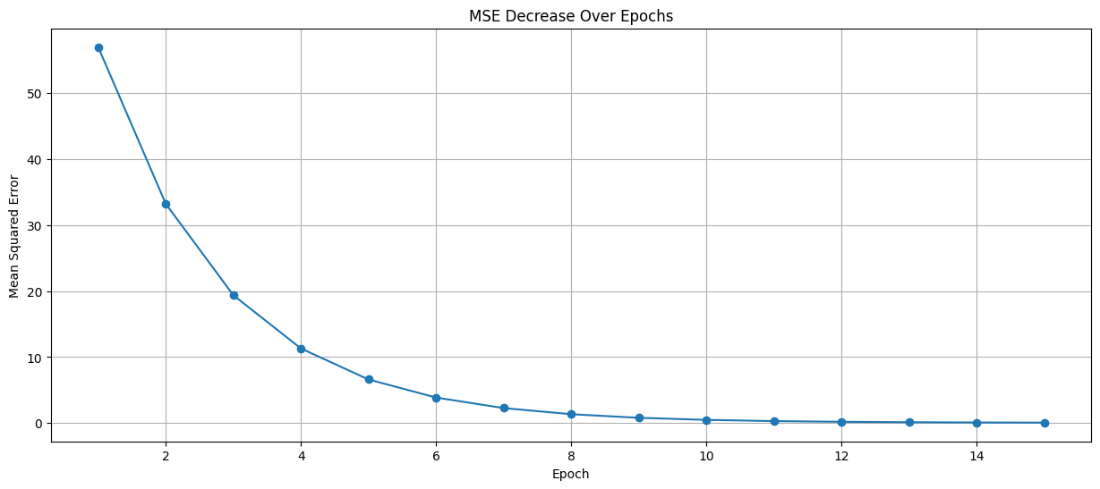
\[= 33.2296 \approx 33.23\]

<blockquote>
  <p>Loss has decreased from 57 → 33.23. The model is learning.</p>
</blockquote>

<hr />

<h3 id="4-calculating-gradients">4. Calculating Gradients</h3>

<h4 id="a-gradient-wrt-weight-w-1">A. Gradient w.r.t Weight (w)</h4>

\[\frac{\partial J}{\partial w}/d_w = \frac{2}{n} \sum_{i=1}^{n} (\hat{y}_i - y_i) x_i\]

\[d_w = \frac{2}{5} [(-2.36 \cdot 1) + (-3.86 \cdot 2) + (-5.36 \cdot 3) + (-6.86 \cdot 4) + (-8.36 \cdot 5)]\]

\[= \frac{2}{5}(-2.36 - 7.72 - 16.08 - 27.44 - 41.8)\]

\[= \frac{2}{5}(-95.4)\]

\[= -38.16\]

<h4 id="b-gradient-wrt-bias-b-1">B. Gradient w.r.t Bias (b)</h4>

\[\frac{\partial J}{\partial b}/d_b = \frac{2}{n} \sum_{i=1}^{n} (\hat{y}_i - y_i)\]

\[= \frac{2}{5} [(-2.36) + (-3.86) + (-5.36) + (-6.86) + (-8.36)]\]

\[= \frac{2}{5} [-2.36 - 3.86 - 5.36 - 6.86 - 8.36]\]

\[= \frac{2}{5}(-26.8)\]

\[= -10.72\]

<hr />

<h3 id="5-updating-parameters">5. Updating Parameters</h3>
<p>\((\eta = 0.01)\)</p>

\[w = w - \eta \cdot d_w\]

\[= 0.5 - 0.01(-38.16)\]

\[= 0.5 + 0.3816\]

\[= 0.8816\]

\[b = b - \eta \cdot d_b\]

\[= 0.14 - 0.01(-10.72)\]

\[= 0.14 + 0.1072\]

\[= 0.2472\]

<blockquote>
  <p>After iteration 2: \((w = 0.8816, b = 0.2472)\)</p>
</blockquote>

<hr />

<h2 id="iteration-3">Iteration 3</h2>

<h3 id="1-making-predictions-1">1. Making Predictions</h3>

<p>Using updated parameters from Iteration 2:</p>

\[w = 0.8816\]

\[b = 0.2472\]

<p>Using the <strong>linear model</strong>:</p>

\[\hat{y} = w \cdot X + b\]

<p>Substituting \((w = 0.8816, b = 0.2472)\):</p>

\[\hat{y} = [0.8816\cdot 1 + 0.2472, \enspace 0.8816\cdot 2 + 0.2472, \enspace 0.8816\cdot 3 + 0.2472, \enspace 0.8816\cdot 4 + 0.2472, \enspace 0.8816\cdot 5 + 0.2472]\]

\[= [0.8816 + 0.2472, \enspace 1.7632 + 0.2472, \enspace 2.6448 + 0.2472, \enspace 3.5264 + 0.2472, \enspace 4.408 + 0.2472]\]

<p>\(= [1.1288, \enspace 2.0104, \enspace 2.892, \enspace 3.7736, \enspace 4.6552]\)
\(= [1.1288, \enspace 2.0104, \enspace 2.892, \enspace 3.7736, \enspace 4.6552]\)</p>

<blockquote>
  <p>The predictions continue moving closer to the actual values.</p>
</blockquote>

<hr />

<h3 id="2-calculating-errors-1">2. Calculating Errors</h3>

\[\text{Error} = \hat{y} - y\]

\[= [1.1288 - 3, \enspace 2.0104 - 5, \enspace 2.892 - 7, \enspace 3.7736 - 9, \enspace 4.6552 - 11]\]

\[= [-1.8712, -2.9896, -4.108, -5.2264, -6.3448]\]

<hr />

<h3 id="3-calculating-loss-mse-1">3. Calculating Loss (MSE)</h3>

\[J(w, b) = \frac{1}{5} \sum (\hat{y}_i - y_i)^2\]

\[= \frac{1}{5} [(-1.8712)^2 + (-2.9896)^2 + (-4.108)^2 + (-5.2264)^2 + (-6.3448)^2]\]

\[= \frac{1}{5} [3.50138944 + 8.93770816 + 16.875664 + 27.31424896 + 40.25447104]\]

\[= \frac{1}{5} [96.8834816] = 19.37669632 \approx 19.38\]

<blockquote>
  <p>Loss has decreased further, showing the model is improving.</p>
</blockquote>

<hr />

<h3 id="4-calculating-gradients-1">4. Calculating Gradients</h3>

<h4 id="a-gradient-wrt-weight-w-2">A. Gradient w.r.t Weight (w)</h4>

\[\frac{\partial J}{\partial w}/d_w = \frac{2}{n} \sum_{i=1}^{n} (\hat{y}_i - y_i) x_i\]

\[d_w = \frac{2}{5} [(-1.8712 \cdot 1) + (-2.9896 \cdot 2) + (-4.108 \cdot 3) + (-5.2264 \cdot 4) + (-6.3448 \cdot 5)]\]

\[= \frac{2}{5}(-1.8712 - 5.9792 - 12.324 - 20.9056 - 31.724)\]

\[= \frac{2}{5}(-72.804) = -29.1216\]

<h4 id="b-gradient-wrt-bias-b-2">B. Gradient w.r.t Bias (b)</h4>

\[\frac{\partial J}{\partial b}/d_b = \frac{2}{n} \sum_{i=1}^{n} (\hat{y}_i - y_i)\]

\[d_b = \frac{2}{5} [(-1.8712) + (-2.9896) + (-4.108) + (-5.2264) + (-6.3448)]\]

\[= \frac{2}{5}(-20.54) = -8.216\]

<hr />

<h3 id="5-updating-parameters-1">5. Updating Parameters</h3>

\[(\eta = 0.01)\]

\[w = w - \eta \cdot d_w\]

\[= 0.8816 - 0.01(-29.1216)\]

\[= 0.8816 + 0.291216\]

\[= 1.172816\]

\[b = b - \eta \cdot d_b\]

\[= 0.2472 - 0.01(-8.216)\]

\[= 0.2472 + 0.08216\]

\[= 0.32936\]

<blockquote>
  <p>After iteration 3: \((w = 1.172816, b = 0.32936)\)</p>
</blockquote>

<hr />

<h2 id="iteration-4">Iteration 4</h2>

<h3 id="1-making-predictions-2">1. Making Predictions</h3>

<p>Using updated parameters from Iteration 3:</p>

\[w = 1.172816\]

\[b = 0.32936\]

<p>Using the <strong>linear model</strong>:</p>

\[\hat{y} = w \cdot X + b\]

<p>Substituting \((w = 1.172816, b = 0.32936)\):</p>

\[\hat{y} = [1.172816\cdot 1 + 0.32936, \enspace 1.172816\cdot 2 + 0.32936, \enspace 1.172816\cdot 3 + 0.32936, \enspace 1.172816\cdot 4 + 0.32936, \enspace 1.172816\cdot 5 + 0.32936]\]

\[= [1.172816 + 0.32936, \enspace 2.345632 + 0.32936, \enspace 3.518448 + 0.32936, \enspace 4.691264 + 0.32936, \enspace 5.86408 + 0.32936]\]

\[= [1.502176, \enspace 2.674992, \enspace 3.847808, \enspace 5.020624, \enspace 6.19344]\]

<blockquote>
  <p>The predictions continue to move closer to the actual values.</p>
</blockquote>

<hr />

<h3 id="2-calculating-errors-2">2. Calculating Errors</h3>

\[\text{Error} = \hat{y} - y\]

\[= [1.502176 - 3, \enspace 2.674992 - 5, \enspace 3.847808 - 7, \enspace 5.020624 - 9, \enspace 6.19344 - 11]\]

\[= [-1.497824, -2.325008, -3.152192, -3.979376, -4.80656]\]

<hr />

<h3 id="3-calculating-loss-mse-2">3. Calculating Loss (MSE)</h3>

\[J(w, b) = \frac{1}{5} \sum (\hat{y}_i - y_i)^2\]

\[= \frac{1}{5} [(-1.497824)^2 + (-2.325008)^2 + (-3.152192)^2 + (-3.979376)^2 + (-4.80656)^2]\]

\[= \frac{1}{5} [2.24347671 + 5.4056622 + 9.93631439 + 15.83543328 + 23.10301879]\]

\[= \frac{1}{5} [56.52390537]\]

\[= 11.30478107 \approx 11.30\]

<blockquote>
  <p>Loss continues decreasing, indicating the model is learning the correct relationship.</p>
</blockquote>

<hr />

<h3 id="4-calculating-gradients-2">4. Calculating Gradients</h3>

<h4 id="a-gradient-wrt-weight-w-3">A. Gradient w.r.t Weight (w)</h4>

\[\frac{\partial J}{\partial w}/d_w = \frac{2}{n} \sum_{i=1}^{n} (\hat{y}_i - y_i) x_i\]

\[d_w = \frac{2}{5} [(-1.497824 \cdot 1) + (-2.325008 \cdot 2) + (-3.152192 \cdot 3) + (-3.979376 \cdot 4) + (-4.80656 \cdot 5)]\]

\[= \frac{2}{5}(-1.497824 - 4.650016 - 9.456576 - 15.917504 - 24.0328)\]

\[= \frac{2}{5}(-55.55472)\]

\[= -22.221888\]

<h4 id="b-gradient-wrt-bias-b-3">B. Gradient w.r.t Bias (b)</h4>

\[\frac{\partial J}{\partial b}/d_b = \frac{2}{n} \sum_{i=1}^{n} (\hat{y}_i - y_i)\]

\[d_b = \frac{2}{5} [(-1.497824) + (-2.325008) + (-3.152192) + (-3.979376) + (-4.80656)]\]

\[= \frac{2}{5}(-15.761)\]

\[= -6.304384\]

<hr />

<h3 id="5-updating-parameters-2">5. Updating Parameters</h3>

\[(\eta = 0.01)\]

\[w = w - \eta \cdot d_w\]

\[= 1.172816 - 0.01(-22.221888)\]

\[= 1.172816 + 0.22221888\]

\[= 1.39503488\]

\[b = b - \eta \cdot d_b\]

\[= 0.32936 - 0.01(-6.304384)\]

\[= 0.32936 + 0.06304384\]

\[= 0.39240384\]

<blockquote>
  <p>After iteration 4: \((w = 1.39503488, b = 0.39240384)\)</p>
</blockquote>

<hr />

<h2 id="iteration-5">Iteration 5</h2>

<h3 id="1-making-predictions-3">1. Making Predictions</h3>

<p>Using updated parameters from Iteration 4:</p>

\[w = 1.39503488\]

\[b = 0.39240384\]

<p>Using the <strong>linear model</strong>:</p>

\[\hat{y} = w \cdot X + b\]

<p>Substituting \((w = 1.39503488, b = 0.39240384)\):</p>

\[\hat{y} = [1.39503488\cdot 1 + 0.39240384, \enspace 1.39503488\cdot 2 + 0.39240384, \enspace 1.39503488\cdot 3 + 0.39240384, \enspace 1.39503488\cdot 4 + 0.39240384, \enspace 1.39503488\cdot 5 + 0.39240384]\]

\[= [1.39503488 + 0.39240384, \enspace 2.79006976 + 0.39240384, \enspace 4.18510464 + 0.39240384, \enspace 5.58013952 + 0.39240384, \enspace 6.9751744 + 0.39240384]\]

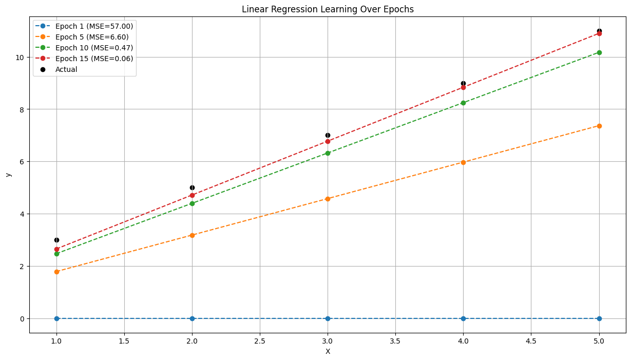
\[= [1.78743872, \enspace 3.1824736, \enspace 4.57750848, \enspace 5.97254336, \enspace 7.36757824]\]

<blockquote>
  <p>The predictions are getting closer to the true values.</p>
</blockquote>

<hr />

<h3 id="2-calculating-errors-3">2. Calculating Errors</h3>

\[\text{Error} = \hat{y} - y\]

\[= [1.78743872 - 3, \enspace 3.1824736 - 5, \enspace 4.57750848 - 7, \enspace 5.97254336 - 9, \enspace 7.36757824 - 11]\]

\[= [-1.21256128, -1.8175264, -2.42249152, -3.02745664, -3.63242176]\]

<hr />

<h3 id="3-calculating-loss-mse-3">3. Calculating Loss (MSE)</h3>

\[J(w, b) = \frac{1}{5} \sum (\hat{y}_i - y_i)^2\]

\[= \frac{1}{5} [(-1.21256128)^2 + (-1.8175264)^2 + (-2.42249152)^2 + (-3.02745664)^2 + (-3.63242176)^2]\]

\[= \frac{1}{5} [1.47030504 + 3.30340191 + 5.86846117 + 9.16548284 + 13.19446689]\]

\[= \frac{1}{5} [33.00211785]\]

\[= 6.60042357 \approx 6.60\]

<blockquote>
  <p>Loss keeps decreasing as the model parameters improve.</p>
</blockquote>

<hr />

<h3 id="4-calculating-gradients-3">4. Calculating Gradients</h3>

<h4 id="a-gradient-wrt-weight-w-4">A. Gradient w.r.t Weight (w)</h4>

\[\frac{\partial J}{\partial w}/d_w = \frac{2}{n} \sum_{i=1}^{n} (\hat{y}_i - y_i) x_i\]

\[d_w = \frac{2}{5} [(-1.21256128 \cdot 1) + (-1.8175264 \cdot 2) + (-2.42249152 \cdot 3) + (-3.02745664 \cdot 4) + (-3.63242176 \cdot 5)]\]

\[= \frac{2}{5}(-1.21256128 - 3.6350528 - 7.26747456 - 12.10982656 - 18.1621088)\]

\[= \frac{2}{5}(-42.387024)\]

\[= -16.9548096\]

<h4 id="b-gradient-wrt-bias-b-4">B. Gradient w.r.t Bias (b)</h4>

\[\frac{\partial J}{\partial b}/d_b = \frac{2}{n} \sum_{i=1}^{n} (\hat{y}_i - y_i)\]

\[d_b = \frac{2}{5} [(-1.21256128) + (-1.8175264) + (-2.42249152) + (-3.02745664) + (-3.63242176)]\]

\[= \frac{2}{5}(-12.1124576)\]

\[= -4.84498304\]

<hr />

<h3 id="5-updating-parameters-3">5. Updating Parameters</h3>

\[(\eta = 0.01)\]

\[w = w - \eta \cdot d_w\]

\[= 1.39503488 - 0.01(-16.9548096)\]

\[= 1.39503488 + 0.169548096\]

\[= 1.564582976\]

\[b = b - \eta \cdot d_b\]

\[= 0.39240384 - 0.01(-4.84498304)\]

\[= 0.39240384 + 0.0484498304\]

\[= 0.4408536704\]

<blockquote>
  <p>After iteration 5: \((w = 1.564582976, b = 0.4408536704)\)</p>
</blockquote>

<hr />

<h2 id="python-implementation">Python Implementation</h2>

<div class="language-py highlighter-rouge"><div class="highlight"><pre class="highlight"><code><span class="kn">import</span> <span class="nn">numpy</span> <span class="k">as</span> <span class="n">np</span>
<span class="kn">import</span> <span class="nn">matplotlib.pyplot</span> <span class="k">as</span> <span class="n">plt</span>

<span class="c1"># Dataset
</span><span class="n">X</span> <span class="o">=</span> <span class="n">np</span><span class="p">.</span><span class="n">array</span><span class="p">([</span><span class="mi">1</span><span class="p">,</span> <span class="mi">2</span><span class="p">,</span> <span class="mi">3</span><span class="p">,</span> <span class="mi">4</span><span class="p">,</span> <span class="mi">5</span><span class="p">],</span> <span class="n">dtype</span><span class="o">=</span><span class="nb">float</span><span class="p">)</span>
<span class="n">y</span> <span class="o">=</span> <span class="n">np</span><span class="p">.</span><span class="n">array</span><span class="p">([</span><span class="mi">3</span><span class="p">,</span> <span class="mi">5</span><span class="p">,</span> <span class="mi">7</span><span class="p">,</span> <span class="mi">9</span><span class="p">,</span> <span class="mi">11</span><span class="p">],</span> <span class="n">dtype</span><span class="o">=</span><span class="nb">float</span><span class="p">)</span>

<span class="c1"># Parameters
</span><span class="n">weights</span> <span class="o">=</span> <span class="mf">0.0</span>
<span class="n">bias</span> <span class="o">=</span> <span class="mf">0.0</span>
<span class="n">learning_rate</span> <span class="o">=</span> <span class="mf">0.01</span>
<span class="n">epochs</span> <span class="o">=</span> <span class="mi">15</span>
<span class="n">n</span> <span class="o">=</span> <span class="nb">len</span><span class="p">(</span><span class="n">X</span><span class="p">)</span>

<span class="c1"># Store MSE for plotting
</span><span class="n">mse_list</span> <span class="o">=</span> <span class="p">[]</span>

<span class="c1"># Print table header
</span><span class="k">print</span><span class="p">(</span><span class="sa">f</span><span class="s">"</span><span class="si">{</span><span class="s">'Epoch'</span><span class="si">:</span><span class="o">^</span><span class="mi">5</span><span class="si">}</span><span class="s"> | </span><span class="si">{</span><span class="s">'Init W'</span><span class="si">:</span><span class="o">^</span><span class="mi">8</span><span class="si">}</span><span class="s"> | </span><span class="si">{</span><span class="s">'Init B'</span><span class="si">:</span><span class="o">^</span><span class="mi">8</span><span class="si">}</span><span class="s"> | </span><span class="si">{</span><span class="s">'Pred y'</span><span class="si">:</span><span class="o">^</span><span class="mi">27</span><span class="si">}</span><span class="s">    | </span><span class="si">{</span><span class="s">'MSE'</span><span class="si">:</span><span class="o">^</span><span class="mi">10</span><span class="si">}</span><span class="s"> | </span><span class="si">{</span><span class="s">'Grad W'</span><span class="si">:</span><span class="o">^</span><span class="mi">10</span><span class="si">}</span><span class="s"> | </span><span class="si">{</span><span class="s">'Grad B'</span><span class="si">:</span><span class="o">^</span><span class="mi">10</span><span class="si">}</span><span class="s"> | </span><span class="si">{</span><span class="s">'Upd W'</span><span class="si">:</span><span class="o">^</span><span class="mi">8</span><span class="si">}</span><span class="s"> | </span><span class="si">{</span><span class="s">'Upd B'</span><span class="si">:</span><span class="o">^</span><span class="mi">8</span><span class="si">}</span><span class="s">"</span><span class="p">)</span>
<span class="k">print</span><span class="p">(</span><span class="s">"-"</span><span class="o">*</span><span class="mi">120</span><span class="p">)</span>

<span class="n">plt</span><span class="p">.</span><span class="n">figure</span><span class="p">(</span><span class="n">figsize</span><span class="o">=</span><span class="p">(</span><span class="mi">15</span><span class="p">,</span><span class="mi">8</span><span class="p">))</span>

<span class="k">for</span> <span class="n">i</span> <span class="ow">in</span> <span class="nb">range</span><span class="p">(</span><span class="n">epochs</span><span class="p">):</span>
    <span class="c1"># Store initial weights/bias for table
</span>    <span class="n">init_w</span> <span class="o">=</span> <span class="n">weights</span>
    <span class="n">init_b</span> <span class="o">=</span> <span class="n">bias</span>
    
    <span class="c1"># Prediction
</span>    <span class="n">y_pred</span> <span class="o">=</span> <span class="n">weights</span> <span class="o">*</span> <span class="n">X</span> <span class="o">+</span> <span class="n">bias</span>
    
    <span class="c1"># MSE
</span>    <span class="n">mse</span> <span class="o">=</span> <span class="n">np</span><span class="p">.</span><span class="n">mean</span><span class="p">((</span><span class="n">y_pred</span> <span class="o">-</span> <span class="n">y</span><span class="p">)</span> <span class="o">**</span> <span class="mi">2</span><span class="p">)</span>
    <span class="n">mse_list</span><span class="p">.</span><span class="n">append</span><span class="p">(</span><span class="n">mse</span><span class="p">)</span>
    
    <span class="c1"># Gradients
</span>    <span class="n">dw</span> <span class="o">=</span> <span class="p">(</span><span class="mi">2</span><span class="o">/</span><span class="n">n</span><span class="p">)</span> <span class="o">*</span> <span class="n">np</span><span class="p">.</span><span class="nb">sum</span><span class="p">((</span><span class="n">y_pred</span> <span class="o">-</span> <span class="n">y</span><span class="p">)</span> <span class="o">*</span> <span class="n">X</span><span class="p">)</span>
    <span class="n">db</span> <span class="o">=</span> <span class="p">(</span><span class="mi">2</span><span class="o">/</span><span class="n">n</span><span class="p">)</span> <span class="o">*</span> <span class="n">np</span><span class="p">.</span><span class="nb">sum</span><span class="p">(</span><span class="n">y_pred</span> <span class="o">-</span> <span class="n">y</span><span class="p">)</span>
    
    <span class="c1"># Update parameters
</span>    <span class="n">weights</span> <span class="o">-=</span> <span class="n">learning_rate</span> <span class="o">*</span> <span class="n">dw</span>
    <span class="n">bias</span> <span class="o">-=</span> <span class="n">learning_rate</span> <span class="o">*</span> <span class="n">db</span>
    
    <span class="c1"># Round predicted values for display
</span>    <span class="n">y_pred_str</span> <span class="o">=</span> <span class="s">"["</span> <span class="o">+</span> <span class="s">", "</span><span class="p">.</span><span class="n">join</span><span class="p">(</span><span class="sa">f</span><span class="s">"</span><span class="si">{</span><span class="n">v</span><span class="si">:</span><span class="p">.</span><span class="mi">2</span><span class="n">f</span><span class="si">}</span><span class="s">"</span> <span class="k">for</span> <span class="n">v</span> <span class="ow">in</span> <span class="n">y_pred</span><span class="p">)</span> <span class="o">+</span> <span class="s">"]"</span>
    
    <span class="c1"># Print table row
</span>    <span class="k">print</span><span class="p">(</span><span class="sa">f</span><span class="s">"</span><span class="si">{</span><span class="n">i</span><span class="o">+</span><span class="mi">1</span><span class="si">:</span><span class="o">^</span><span class="mi">5</span><span class="si">}</span><span class="s"> | </span><span class="si">{</span><span class="n">init_w</span><span class="si">:</span><span class="o">^</span><span class="mf">8.4</span><span class="n">f</span><span class="si">}</span><span class="s"> | </span><span class="si">{</span><span class="n">init_b</span><span class="si">:</span><span class="o">^</span><span class="mf">8.4</span><span class="n">f</span><span class="si">}</span><span class="s"> | </span><span class="si">{</span><span class="n">y_pred_str</span><span class="si">:</span><span class="o">^</span><span class="mi">27</span><span class="si">}</span><span class="s"> | </span><span class="si">{</span><span class="n">mse</span><span class="si">:</span><span class="o">^</span><span class="mf">10.4</span><span class="n">f</span><span class="si">}</span><span class="s"> | </span><span class="si">{</span><span class="n">dw</span><span class="si">:</span><span class="o">^</span><span class="mf">10.4</span><span class="n">f</span><span class="si">}</span><span class="s"> | </span><span class="si">{</span><span class="n">db</span><span class="si">:</span><span class="o">^</span><span class="mf">10.4</span><span class="n">f</span><span class="si">}</span><span class="s"> | </span><span class="si">{</span><span class="n">weights</span><span class="si">:</span><span class="o">^</span><span class="mf">8.4</span><span class="n">f</span><span class="si">}</span><span class="s"> | </span><span class="si">{</span><span class="n">bias</span><span class="si">:</span><span class="o">^</span><span class="mf">8.4</span><span class="n">f</span><span class="si">}</span><span class="s">"</span><span class="p">)</span>
    
    <span class="c1"># Plot predictions every 5 epochs + first epoch
</span>    <span class="k">if</span> <span class="p">(</span><span class="n">i</span><span class="o">+</span><span class="mi">1</span><span class="p">)</span> <span class="o">%</span> <span class="mi">5</span> <span class="o">==</span> <span class="mi">0</span> <span class="ow">or</span> <span class="n">i</span> <span class="o">==</span> <span class="mi">0</span><span class="p">:</span>
        <span class="n">plt</span><span class="p">.</span><span class="n">plot</span><span class="p">(</span><span class="n">X</span><span class="p">,</span> <span class="n">y_pred</span><span class="p">,</span> <span class="n">marker</span><span class="o">=</span><span class="s">'o'</span><span class="p">,</span> <span class="n">linestyle</span><span class="o">=</span><span class="s">'--'</span><span class="p">,</span> <span class="n">label</span><span class="o">=</span><span class="sa">f</span><span class="s">'Epoch </span><span class="si">{</span><span class="n">i</span><span class="o">+</span><span class="mi">1</span><span class="si">}</span><span class="s"> (MSE=</span><span class="si">{</span><span class="n">mse</span><span class="si">:</span><span class="p">.</span><span class="mi">2</span><span class="n">f</span><span class="si">}</span><span class="s">)'</span><span class="p">)</span>

<span class="c1"># Plot actual data
</span><span class="n">plt</span><span class="p">.</span><span class="n">scatter</span><span class="p">(</span><span class="n">X</span><span class="p">,</span> <span class="n">y</span><span class="p">,</span> <span class="n">color</span><span class="o">=</span><span class="s">'black'</span><span class="p">,</span> <span class="n">label</span><span class="o">=</span><span class="s">'Actual'</span><span class="p">)</span>
<span class="n">plt</span><span class="p">.</span><span class="n">xlabel</span><span class="p">(</span><span class="s">'X'</span><span class="p">)</span>
<span class="n">plt</span><span class="p">.</span><span class="n">ylabel</span><span class="p">(</span><span class="s">'y'</span><span class="p">)</span>
<span class="n">plt</span><span class="p">.</span><span class="n">title</span><span class="p">(</span><span class="s">'Linear Regression Learning Over Epochs'</span><span class="p">)</span>
<span class="n">plt</span><span class="p">.</span><span class="n">legend</span><span class="p">()</span>
<span class="n">plt</span><span class="p">.</span><span class="n">grid</span><span class="p">(</span><span class="bp">True</span><span class="p">)</span>
<span class="n">plt</span><span class="p">.</span><span class="n">show</span><span class="p">()</span>

<span class="c1"># Plot MSE over epochs
</span><span class="n">plt</span><span class="p">.</span><span class="n">figure</span><span class="p">(</span><span class="n">figsize</span><span class="o">=</span><span class="p">(</span><span class="mi">15</span><span class="p">,</span><span class="mi">6</span><span class="p">))</span>
<span class="n">plt</span><span class="p">.</span><span class="n">plot</span><span class="p">(</span><span class="nb">range</span><span class="p">(</span><span class="mi">1</span><span class="p">,</span> <span class="n">epochs</span><span class="o">+</span><span class="mi">1</span><span class="p">),</span> <span class="n">mse_list</span><span class="p">,</span> <span class="n">marker</span><span class="o">=</span><span class="s">'o'</span><span class="p">,</span> <span class="n">linestyle</span><span class="o">=</span><span class="s">'-'</span><span class="p">)</span>
<span class="n">plt</span><span class="p">.</span><span class="n">xlabel</span><span class="p">(</span><span class="s">'Epoch'</span><span class="p">)</span>
<span class="n">plt</span><span class="p">.</span><span class="n">ylabel</span><span class="p">(</span><span class="s">'Mean Squared Error'</span><span class="p">)</span>
<span class="n">plt</span><span class="p">.</span><span class="n">title</span><span class="p">(</span><span class="s">'MSE Decrease Over Epochs'</span><span class="p">)</span>
<span class="n">plt</span><span class="p">.</span><span class="n">grid</span><span class="p">(</span><span class="bp">True</span><span class="p">)</span>
<span class="n">plt</span><span class="p">.</span><span class="n">show</span><span class="p">()</span>
</code></pre></div></div>

<p>Oputput:</p>
<div class="language-plaintext highlighter-rouge"><div class="highlight"><pre class="highlight"><code>Epoch |  Init W  |  Init B  |           Pred y               |    MSE     |   Grad W   |   Grad B   |  Upd W   |  Upd B  
------------------------------------------------------------------------------------------------------------------------
  1   |  0.0000  |  0.0000  | [0.00, 0.00, 0.00, 0.00, 0.00] |  57.0000   |  -50.0000  |  -14.0000  |  0.5000  |  0.1400 
  2   |  0.5000  |  0.1400  | [0.64, 1.14, 1.64, 2.14, 2.64] |  33.2296   |  -38.1600  |  -10.7200  |  0.8816  |  0.2472 
  3   |  0.8816  |  0.2472  | [1.13, 2.01, 2.89, 3.77, 4.66] |  19.3773   |  -29.1216  |  -8.2160   |  1.1728  |  0.3294 
  4   |  1.1728  |  0.3294  | [1.50, 2.67, 3.85, 5.02, 6.19] |  11.3048   |  -22.2219  |  -6.3044   |  1.3950  |  0.3924 
  5   |  1.3950  |  0.3924  | [1.79, 3.18, 4.58, 5.97, 7.37] |   6.6004   |  -16.9548  |  -4.8450   |  1.5646  |  0.4409 
  6   |  1.5646  |  0.4409  | [2.01, 3.57, 5.13, 6.70, 8.26] |   3.8589   |  -12.9341  |  -3.7308   |  1.6939  |  0.4782 
  7   |  1.6939  |  0.4782  | [2.17, 3.87, 5.56, 7.25, 8.95] |   2.2612   |  -9.8647   |  -2.8801   |  1.7926  |  0.5070 
  8   |  1.7926  |  0.5070  | [2.30, 4.09, 5.88, 7.68, 9.47] |   1.3300   |  -7.5217   |  -2.2307   |  1.8678  |  0.5293 
  9   |  1.8678  |  0.5293  | [2.40, 4.26, 6.13, 8.00, 9.87] |   0.7873   |  -5.7331   |  -1.7347   |  1.9251  |  0.5466 
 10   |  1.9251  |  0.5466  | [2.47, 4.40, 6.32, 8.25, 10.17] |   0.4709   |  -4.3677   |  -1.3561   |  1.9688  |  0.5602 
 11   |  1.9688  |  0.5602  | [2.53, 4.50, 6.47, 8.44, 10.40] |   0.2865   |  -3.3254   |  -1.0669   |  2.0020  |  0.5708 
 12   |  2.0020  |  0.5708  | [2.57, 4.57, 6.58, 8.58, 10.58] |   0.1789   |  -2.5298   |  -0.8460   |  2.0273  |  0.5793 
 13   |  2.0273  |  0.5793  | [2.61, 4.63, 6.66, 8.69, 10.72] |   0.1162   |  -1.9225   |  -0.6773   |  2.0466  |  0.5861 
 14   |  2.0466  |  0.5861  | [2.63, 4.68, 6.73, 8.77, 10.82] |   0.0795   |  -1.4589   |  -0.5484   |  2.0612  |  0.5916 
 15   |  2.0612  |  0.5916  | [2.65, 4.71, 6.78, 8.84, 10.90] |   0.0581   |  -1.1051   |  -0.4499   |  2.0722  |  0.5961 
</code></pre></div></div>

<p><strong>Charts</strong>:<br />
<img src="/assets/images/machine-learning/supervised-learning/linear-regression-learning-over-epochs.png" alt="Linear Regression Learning Over Epochs" /></p>

<p><img src="/assets/images/machine-learning/supervised-learning/mse-decrease-over-epochs.png" alt="MSE Decrease Over Epochs" /></p>]]></content><author><name>Dipak Pulami Magar</name></author><category term="machine-learning" /><category term="supervised" /><category term="regression" /><summary type="html"><![CDATA[A Complete Guide with Example and Python Code]]></summary></entry><entry><title type="html">Bag of Words (BoW)</title><link href="https://dpm24800.github.io/deep-learning/nlp/2026/02/25/bag-of-words.html" rel="alternate" type="text/html" title="Bag of Words (BoW)" /><published>2026-02-25T07:27:45+00:00</published><updated>2026-02-25T07:27:45+00:00</updated><id>https://dpm24800.github.io/deep-learning/nlp/2026/02/25/bag-of-words</id><content type="html" xml:base="https://dpm24800.github.io/deep-learning/nlp/2026/02/25/bag-of-words.html"><![CDATA[<h2 id="overview">Overview</h2>
<ul>
  <li>Bag of Words is a feature extraction method that converts text into a vector of word counts.</li>
  <li>It is a simple way to represent text as numbers by counting how many times each word appears in a document.</li>
  <li>It <strong>ignores grammar and word order</strong> and only keeps:
    <ul>
      <li>which words appear, and</li>
      <li>how often they appear.</li>
    </ul>
  </li>
  <li>This is the base idea behind models like text classification, spam detection, and sentiment analysis.</li>
</ul>

<h2 id="example">Example</h2>
<p>Suppose you have these documents:</p>
<ul>
  <li>D1: <code class="language-plaintext highlighter-rouge">"Blue sky"</code></li>
  <li>D2: <code class="language-plaintext highlighter-rouge">"Bright sun today"</code></li>
  <li>D3: <code class="language-plaintext highlighter-rouge">"Bright sun sky"</code></li>
  <li>D4: <code class="language-plaintext highlighter-rouge">"Can see bright sun shining"</code></li>
</ul>

<h3 id="step-1-build-the-vocabulary-all-unique-words">Step 1: Build the vocabulary (all unique words)</h3>
<p>Remove stop words (common words that don’t add much meaning).</p>

<p>Then, build the vocabulary from the remaining words:</p>

<ul>
  <li>Vocabulary: <code class="language-plaintext highlighter-rouge">[blue, sky, bright, sun, today, can, see, shining]</code></li>
  <li>Sorted alphabetically:
<code class="language-plaintext highlighter-rouge">[blue, bright, can, see, shining, sky, sun, today]</code></li>
</ul>

<h3 id="step-2-represent-each-document-as-word-counts">Step 2: Represent each document as word counts</h3>

<table>
  <thead>
    <tr>
      <th>Sentence</th>
      <th>blue</th>
      <th>bright</th>
      <th>can</th>
      <th>see</th>
      <th>shining</th>
      <th>sky</th>
      <th>sun</th>
      <th>today</th>
    </tr>
  </thead>
  <tbody>
    <tr>
      <td>D1</td>
      <td>1</td>
      <td>0</td>
      <td>0</td>
      <td>0</td>
      <td>0</td>
      <td>1</td>
      <td>0</td>
      <td>0</td>
    </tr>
    <tr>
      <td>D2</td>
      <td>0</td>
      <td>1</td>
      <td>0</td>
      <td>0</td>
      <td>0</td>
      <td>0</td>
      <td>1</td>
      <td>1</td>
    </tr>
    <tr>
      <td>D3</td>
      <td>0</td>
      <td>1</td>
      <td>0</td>
      <td>0</td>
      <td>0</td>
      <td>1</td>
      <td>1</td>
      <td>0</td>
    </tr>
    <tr>
      <td>D4</td>
      <td>0</td>
      <td>1</td>
      <td>1</td>
      <td>1</td>
      <td>1</td>
      <td>0</td>
      <td>1</td>
      <td>0</td>
    </tr>
  </tbody>
</table>

<p>So:</p>
<ul>
  <li><code class="language-plaintext highlighter-rouge">D1</code> → <code class="language-plaintext highlighter-rouge">[1, 0, 0, 0, 0, 1, 0, 0]</code></li>
  <li><code class="language-plaintext highlighter-rouge">D2</code> → <code class="language-plaintext highlighter-rouge">[0, 1, 0, 0, 0, 0, 1, 1]</code></li>
  <li><code class="language-plaintext highlighter-rouge">D3</code> → <code class="language-plaintext highlighter-rouge">[0, 1, 0, 0, 0, 1, 1, 0]</code></li>
  <li><code class="language-plaintext highlighter-rouge">D4</code> → <code class="language-plaintext highlighter-rouge">[0, 1, 1, 1, 1, 0, 1, 0]</code></li>
</ul>

<p>This numeric vector is the <strong>Bag of Words representation</strong>.</p>

<h2 id="key-points">Key points</h2>
<ul>
  <li>Word order is ignored:
    <ul>
      <li>“bright sun today” gives the same vector as “today bright sun”.</li>
    </ul>
  </li>
  <li>Only frequency matters.</li>
  <li>Very easy to compute and widely used in basic NLP and ML models.</li>
</ul>

<h2 id="in-one-line">In one line</h2>
<blockquote>
  <p>Bag of Words = vocabulary of all words + frequency of each word in a text.</p>
</blockquote>

<h2 id="python-implementation">Python implementation</h2>
<div class="language-py highlighter-rouge"><div class="highlight"><pre class="highlight"><code><span class="kn">from</span> <span class="nn">sklearn.feature_extraction.text</span> <span class="kn">import</span> <span class="n">CountVectorizer</span>

<span class="c1"># Sample documents
</span><span class="n">documents</span> <span class="o">=</span> <span class="p">[</span>
    <span class="s">"Blue sky"</span><span class="p">,</span>
    <span class="s">"Bright sun today"</span><span class="p">,</span>
    <span class="s">"Bright sun sky"</span><span class="p">,</span>
    <span class="s">"Can see bright sun shining"</span>
<span class="p">]</span>

<span class="c1"># Create Bag of Words representation
</span><span class="n">vectorizer</span> <span class="o">=</span> <span class="n">CountVectorizer</span><span class="p">()</span>
<span class="n">X</span> <span class="o">=</span> <span class="n">vectorizer</span><span class="p">.</span><span class="n">fit_transform</span><span class="p">(</span><span class="n">documents</span><span class="p">)</span>

<span class="c1"># Get feature names (vocabulary)
# Vocabulary should be fitted or provided beforehand
</span><span class="n">feature_names</span> <span class="o">=</span> <span class="n">vectorizer</span><span class="p">.</span><span class="n">get_feature_names_out</span><span class="p">()</span> 

<span class="k">print</span><span class="p">(</span><span class="s">"Vocabulary:"</span><span class="p">,</span> <span class="n">feature_names</span><span class="p">)</span>
<span class="k">print</span><span class="p">(</span><span class="s">"</span><span class="se">\n</span><span class="s">Document vectors:"</span><span class="p">)</span>
<span class="k">print</span><span class="p">(</span><span class="n">X</span><span class="p">.</span><span class="n">toarray</span><span class="p">())</span>
</code></pre></div></div>

<p><strong>Output:</strong></p>
<div class="language-text highlighter-rouge"><div class="highlight"><pre class="highlight"><code>Vocabulary: ['blue' 'bright' 'can' 'see' 'shining' 'sky' 'sun' 'today']

Document vectors:
[[1 0 0 0 0 1 0 0]
 [0 1 0 0 0 0 1 1]
 [0 1 0 0 0 1 1 0]
 [0 1 1 1 1 0 1 0]]
</code></pre></div></div>]]></content><author><name>Dipak Pulami Magar</name></author><category term="deep-learning" /><category term="nlp" /><summary type="html"><![CDATA[Overview Bag of Words is a feature extraction method that converts text into a vector of word counts. It is a simple way to represent text as numbers by counting how many times each word appears in a document. It ignores grammar and word order and only keeps: which words appear, and how often they appear. This is the base idea behind models like text classification, spam detection, and sentiment analysis.]]></summary></entry><entry><title type="html">Term Frequency – Inverse Document Frequency (TF-IDF)</title><link href="https://dpm24800.github.io/deep-learning/nlp/2026/02/25/tf-idf.html" rel="alternate" type="text/html" title="Term Frequency – Inverse Document Frequency (TF-IDF)" /><published>2026-02-25T07:27:45+00:00</published><updated>2026-02-25T07:27:45+00:00</updated><id>https://dpm24800.github.io/deep-learning/nlp/2026/02/25/tf-idf</id><content type="html" xml:base="https://dpm24800.github.io/deep-learning/nlp/2026/02/25/tf-idf.html"><![CDATA[<h2 id="overview">Overview</h2>
<ul>
  <li><strong>TF-IDF</strong> is a feature extraction method that reflects how important a word is in a document relative to a collection of documents (corpus).</li>
  <li>
    <p>It combines two ideas:</p>

    <ul>
      <li><strong>Term Frequency (TF):</strong> How often a word appears in a document.</li>
      <li><strong>Inverse Document Frequency (IDF):</strong> How unique or rare the word is across all documents.</li>
    </ul>
  </li>
  <li>Unlike Bag of Words, TF-IDF <strong>reduces the weight of common words</strong> and gives higher weight to rare but meaningful words.</li>
  <li>TF-IDF is widely used in text mining, search engines, and information retrieval.</li>
</ul>

<h2 id="example">Example</h2>

<p>Suppose you have these documents:</p>

<ul>
  <li>D1: <code class="language-plaintext highlighter-rouge">"Blue sky"</code></li>
  <li>D2: <code class="language-plaintext highlighter-rouge">"Bright sun today"</code></li>
  <li>D3: <code class="language-plaintext highlighter-rouge">"Bright sun sky"</code></li>
  <li>D4: <code class="language-plaintext highlighter-rouge">"Can see bright sun shining"</code></li>
</ul>

<h3 id="step-1-compute-term-frequency-tf">Step 1: Compute Term Frequency (TF)</h3>

<p>TF is the count of a word in a document divided by the total number of words in that document.</p>

\[\text{TF}(word, document) = \frac{\text{Count of word in document}}{\text{Total words in document}}\]

<table>
  <thead>
    <tr>
      <th>Document</th>
      <th>blue</th>
      <th>bright</th>
      <th>can</th>
      <th>see</th>
      <th>shining</th>
      <th>sky</th>
      <th>sun</th>
      <th>today</th>
    </tr>
  </thead>
  <tbody>
    <tr>
      <td>D1</td>
      <td>1/2</td>
      <td>0</td>
      <td>0</td>
      <td>0</td>
      <td>0</td>
      <td>1/2</td>
      <td>0</td>
      <td>0</td>
    </tr>
    <tr>
      <td>D2</td>
      <td>0</td>
      <td>1/3</td>
      <td>0</td>
      <td>0</td>
      <td>0</td>
      <td>0</td>
      <td>1/3</td>
      <td>1/3</td>
    </tr>
    <tr>
      <td>D3</td>
      <td>0</td>
      <td>1/3</td>
      <td>0</td>
      <td>0</td>
      <td>0</td>
      <td>1/3</td>
      <td>1/3</td>
      <td>0</td>
    </tr>
    <tr>
      <td>D4</td>
      <td>0</td>
      <td>1/5</td>
      <td>1/5</td>
      <td>1/5</td>
      <td>1/5</td>
      <td>0</td>
      <td>1/5</td>
      <td>0</td>
    </tr>
  </tbody>
</table>

<h3 id="step-2-compute-inverse-document-frequency-idf">Step 2: Compute Inverse Document Frequency (IDF)</h3>

<p>IDF measures how unique a word is across all documents:</p>

\[\text{IDF}(word) = \log\frac{\text{Total documents}}{\text{Number of documents containing the word}}\]

<p>For our example (4 documents):</p>

<table>
  <thead>
    <tr>
      <th>Metric</th>
      <th>blue</th>
      <th>bright</th>
      <th>can</th>
      <th>see</th>
      <th>shining</th>
      <th>sky</th>
      <th>sun</th>
      <th>today</th>
    </tr>
  </thead>
  <tbody>
    <tr>
      <td>DF</td>
      <td>1</td>
      <td>3</td>
      <td>1</td>
      <td>1</td>
      <td>1</td>
      <td>2</td>
      <td>3</td>
      <td>1</td>
    </tr>
    <tr>
      <td>IDF = log(4/DF)</td>
      <td>1.386</td>
      <td>0.287</td>
      <td>1.386</td>
      <td>1.386</td>
      <td>1.386</td>
      <td>0.693</td>
      <td>0.287</td>
      <td>1.386</td>
    </tr>
  </tbody>
</table>

<h3 id="step-3-compute-tf-idf">Step 3: Compute TF-IDF</h3>

<p>Multiply TF by IDF for each word in each document:</p>

<table>
  <thead>
    <tr>
      <th>Document</th>
      <th>blue</th>
      <th>bright</th>
      <th>can</th>
      <th>see</th>
      <th>shining</th>
      <th>sky</th>
      <th>sun</th>
      <th>today</th>
    </tr>
  </thead>
  <tbody>
    <tr>
      <td>D1</td>
      <td>0.693</td>
      <td>0</td>
      <td>0</td>
      <td>0</td>
      <td>0</td>
      <td>0.347</td>
      <td>0</td>
      <td>0</td>
    </tr>
    <tr>
      <td>D2</td>
      <td>0</td>
      <td>0.096</td>
      <td>0</td>
      <td>0</td>
      <td>0</td>
      <td>0</td>
      <td>0.096</td>
      <td>0.462</td>
    </tr>
    <tr>
      <td>D3</td>
      <td>0</td>
      <td>0.096</td>
      <td>0</td>
      <td>0</td>
      <td>0</td>
      <td>0.231</td>
      <td>0.096</td>
      <td>0</td>
    </tr>
    <tr>
      <td>D4</td>
      <td>0</td>
      <td>0.057</td>
      <td>0.277</td>
      <td>0.277</td>
      <td>0.277</td>
      <td>0</td>
      <td>0.057</td>
      <td>0</td>
    </tr>
  </tbody>
</table>

<p>Now each document has a <strong>TF-IDF vector</strong>, showing the importance of words, not just frequency.</p>

<h2 id="key-points">Key points</h2>

<ul>
  <li>Common words like “sun” or “bright” get <strong>lower weight</strong>.</li>
  <li>Rare or unique words like “blue” or “can” get <strong>higher weight</strong>.</li>
  <li>TF-IDF is very effective for search engines, text similarity, and document clustering.</li>
</ul>

<h2 id="in-one-line">In one line</h2>
<blockquote>
  <p>TF-IDF = Term Frequency × Inverse Document Frequency (importance of a word in a document relative to corpus).</p>
</blockquote>

<h2 id="python-implementation">Python implementation</h2>

<div class="language-py highlighter-rouge"><div class="highlight"><pre class="highlight"><code><span class="kn">from</span> <span class="nn">sklearn.feature_extraction.text</span> <span class="kn">import</span> <span class="n">TfidfVectorizer</span>

<span class="c1"># Sample documents
</span><span class="n">documents</span> <span class="o">=</span> <span class="p">[</span>
    <span class="s">"Blue sky"</span><span class="p">,</span>
    <span class="s">"Bright sun today"</span><span class="p">,</span>
    <span class="s">"Bright sun sky"</span><span class="p">,</span>
    <span class="s">"Can see bright sun shining"</span>
<span class="p">]</span>

<span class="c1"># Create TF-IDF representation
</span><span class="n">vectorizer</span> <span class="o">=</span> <span class="n">TfidfVectorizer</span><span class="p">()</span>
<span class="n">X</span> <span class="o">=</span> <span class="n">vectorizer</span><span class="p">.</span><span class="n">fit_transform</span><span class="p">(</span><span class="n">documents</span><span class="p">)</span>

<span class="c1"># Get feature names (vocabulary)
</span><span class="n">feature_names</span> <span class="o">=</span> <span class="n">vectorizer</span><span class="p">.</span><span class="n">get_feature_names_out</span><span class="p">()</span> 

<span class="k">print</span><span class="p">(</span><span class="s">"Vocabulary:"</span><span class="p">,</span> <span class="n">feature_names</span><span class="p">)</span>
<span class="k">print</span><span class="p">(</span><span class="s">"</span><span class="se">\n</span><span class="s">TF-IDF matrix:"</span><span class="p">)</span>
<span class="k">print</span><span class="p">(</span><span class="n">X</span><span class="p">.</span><span class="n">toarray</span><span class="p">())</span>
</code></pre></div></div>

<p><strong>Output (approx.):</strong></p>

<div class="language-text highlighter-rouge"><div class="highlight"><pre class="highlight"><code>Vocabulary: ['blue' 'bright' 'can' 'see' 'shining' 'sky' 'sun' 'today']

TF-IDF matrix:
[[0.693 0.    0.    0.    0.    0.693 0.    0.   ]
 [0.    0.096 0.    0.    0.    0.    0.096 0.462]
 [0.    0.096 0.    0.    0.    0.231 0.096 0.   ]
 [0.    0.057 0.277 0.277 0.277 0.    0.057 0.   ]]
</code></pre></div></div>]]></content><author><name>Dipak Pulami Magar</name></author><category term="deep-learning" /><category term="nlp" /><summary type="html"><![CDATA[Overview TF-IDF is a feature extraction method that reflects how important a word is in a document relative to a collection of documents (corpus). It combines two ideas:]]></summary></entry><entry><title type="html">Changing case in VS Code</title><link href="https://dpm24800.github.io/vscode/2026/02/08/changing-case.html" rel="alternate" type="text/html" title="Changing case in VS Code" /><published>2026-02-08T04:27:45+00:00</published><updated>2026-02-08T04:27:45+00:00</updated><id>https://dpm24800.github.io/vscode/2026/02/08/changing-case</id><content type="html" xml:base="https://dpm24800.github.io/vscode/2026/02/08/changing-case.html"><![CDATA[<p><strong>VS Code does have a “sentence case” option</strong>, but <strong>not by default</strong>.</p>

<h3 id="built-in-options-default">Built-in options (default)</h3>

<p>VS Code only includes:</p>

<ul>
  <li><strong>Uppercase</strong></li>
  <li><strong>Lowercase</strong></li>
  <li><strong>Title Case</strong></li>
</ul>

<p>You can access them via:</p>

<ul>
  <li><strong>Windows/Linux:</strong> <code class="language-plaintext highlighter-rouge">Ctrl + Shift + P</code></li>
  <li><strong>macOS:</strong> <code class="language-plaintext highlighter-rouge">Cmd + Shift + P</code>
→ type <strong>“Transform to…”</strong></li>
</ul>

<p>You won’t see <strong>Sentence Case</strong> there.</p>

<hr />

<h3 id="how-to-get-sentence-case-in-vs-code">How to get Sentence Case in VS Code</h3>

<h4 id="ption-1-install-an-extension-recommended">ption 1: Install an extension (recommended)</h4>

<p>Install <strong>“Change Case”</strong> extension.</p>

<p><strong>Steps:</strong></p>

<ol>
  <li>Open Extensions (<code class="language-plaintext highlighter-rouge">Ctrl + Shift + X</code>)</li>
  <li>Search for <strong>Change Case</strong></li>
  <li>Install it</li>
  <li>Select your text</li>
  <li>Press <code class="language-plaintext highlighter-rouge">Ctrl + Shift + P</code></li>
  <li>Choose <strong>Change Case → Sentence case</strong></li>
</ol>

<p>This converts text like:</p>

<div class="language-plaintext highlighter-rouge"><div class="highlight"><pre class="highlight"><code>this is a test. this is another test.
</code></pre></div></div>

<div class="language-plaintext highlighter-rouge"><div class="highlight"><pre class="highlight"><code>This is a test. This is another test.
</code></pre></div></div>

<hr />

<h4 id="ption-2-keyboard-shortcut-after-extension">ption 2: Keyboard shortcut (after extension)</h4>

<p>Once installed, you can bind a shortcut:</p>

<ul>
  <li>Go to <strong>Keyboard Shortcuts</strong></li>
  <li>Search for <code class="language-plaintext highlighter-rouge">sentence case</code></li>
  <li>Assign your own key combo</li>
</ul>

<hr />

<h3 id="if-you-want-a-quick-workaround-no-extension">If you want a quick workaround (no extension)</h3>

<p>You can:</p>

<ul>
  <li>Convert to <strong>lowercase</strong></li>
  <li>Manually capitalize the first letter</li>
</ul>

<p>…but this <strong>won’t handle multiple sentences correctly</strong>.</p>

<!-- ---

### Recommendation (especially if you write/code a lot)

Use the **Change Case** extension — lightweight, fast, and very useful for documentation, comments, and markdown.

If you want, I can also:

* Show how to do this with **regex**
* Create a **custom VS Code macro**
* Suggest **other writing-friendly extensions**

Just tell me  -->]]></content><author><name>Dipak Pulami Magar</name></author><category term="vscode" /><summary type="html"><![CDATA[VS Code does have a “sentence case” option, but not by default.]]></summary></entry><entry><title type="html">5 CSS Frameworks For Web Developers</title><link href="https://dpm24800.github.io/css/2026/02/08/css-frameworks-for-web-developers.html" rel="alternate" type="text/html" title="5 CSS Frameworks For Web Developers" /><published>2026-02-08T04:27:45+00:00</published><updated>2026-02-08T04:27:45+00:00</updated><id>https://dpm24800.github.io/css/2026/02/08/css-frameworks-for-web-developers</id><content type="html" xml:base="https://dpm24800.github.io/css/2026/02/08/css-frameworks-for-web-developers.html"><![CDATA[<h3 id="1-bootstrap">1. Bootstrap</h3>
<p>Bootstrap offers a robust collection of CSS and JavaScript components, such as its grid system and responsive UI components.</p>

<h3 id="2-bulma">2. Bulma</h3>
<p>Bulma is a modern CSS framework based on Flexbox known for its simplicity, clean syntax, and ease of use.</p>

<h3 id="3-foundation">3. Foundation</h3>
<p>Foundation Features a responsive grid system, a wide range of UI components, and advanced features like interchangeable layouts and modular architecture. Foundation is the closest alternative to Bootstrap.</p>

<h3 id="4-tailwind-css">4. Tailwind CSS</h3>
<p>Tailwind CSS is a utility-first CSS framework that provides low-level utility classes to style web applications. As a utility-first framework, Tailwind abstracts from the constraints of a component-based framework, for example, Bootstrap.</p>

<h3 id="5-material-ui">5. Material UI</h3>
<p>Material UI is a component-based CSS framework for building user interfaces in React applications. It is based on Google’s open- source design system, Material Design, and provides a rich collection of pre-built components and styles.</p>]]></content><author><name>Dipak Pulami Magar</name></author><category term="css" /><summary type="html"><![CDATA[1. Bootstrap Bootstrap offers a robust collection of CSS and JavaScript components, such as its grid system and responsive UI components.]]></summary></entry><entry><title type="html">CSS Positioning</title><link href="https://dpm24800.github.io/css/2026/02/08/css-positioning.html" rel="alternate" type="text/html" title="CSS Positioning" /><published>2026-02-08T04:27:45+00:00</published><updated>2026-02-08T04:27:45+00:00</updated><id>https://dpm24800.github.io/css/2026/02/08/css-positioning</id><content type="html" xml:base="https://dpm24800.github.io/css/2026/02/08/css-positioning.html"><![CDATA[<!-- 
position: static; 
postition: relative;
position: absolute;
postion: sticky;
position: fixed;


# Centering Items
Centering a div in css is now too easy with positions. -->

<p>CSS positioning controls the placement of elements on a web page, allowing developers to override the normal document flow. The core property is <code class="language-plaintext highlighter-rouge">position</code>, which accepts five main values: <code class="language-plaintext highlighter-rouge">static</code>, <code class="language-plaintext highlighter-rouge">relative</code>, <code class="language-plaintext highlighter-rouge">absolute</code>, <code class="language-plaintext highlighter-rouge">fixed</code>, and <code class="language-plaintext highlighter-rouge">sticky</code>.</p>

<p>The <code class="language-plaintext highlighter-rouge">top</code>, <code class="language-plaintext highlighter-rouge">right</code>, <code class="language-plaintext highlighter-rouge">bottom</code>, and <code class="language-plaintext highlighter-rouge">left</code> properties are then used to specify the final location, but they behave differently depending on the <code class="language-plaintext highlighter-rouge">position</code> value.</p>

<h2 id="types-of-css-positioning">Types of CSS Positioning</h2>
<ul>
  <li><strong><code class="language-plaintext highlighter-rouge">static</code></strong>: This is the <strong>default</strong> value for all elements. Elements are positioned according to the normal flow of the page and the <code class="language-plaintext highlighter-rouge">top</code>, <code class="language-plaintext highlighter-rouge">right</code>, <code class="language-plaintext highlighter-rouge">bottom</code>, and <code class="language-plaintext highlighter-rouge">left</code> properties have <strong>no effect</strong>.</li>
  <li><strong><code class="language-plaintext highlighter-rouge">relative</code></strong>: The element remains in the normal flow but can be offset from its original position using <code class="language-plaintext highlighter-rouge">top</code>, <code class="language-plaintext highlighter-rouge">right</code>, <code class="language-plaintext highlighter-rouge">bottom</code>, or <code class="language-plaintext highlighter-rouge">left</code>. The space the element would have occupied is preserved, and the offset does not affect the position of other elements.</li>
  <li><strong><code class="language-plaintext highlighter-rouge">absolute</code></strong>: The element is <strong>removed entirely from the normal document flow</strong>. It is then positioned relative to its <em>nearest positioned ancestor</em> (any ancestor with a position other than <code class="language-plaintext highlighter-rouge">static</code>). If no such ancestor exists, it is positioned relative to the initial containing block (usually the <code class="language-plaintext highlighter-rouge">&lt;html&gt;</code> element/viewport). Other elements on the page will behave as if the absolutely positioned element does not exist.</li>
  <li><strong><code class="language-plaintext highlighter-rouge">fixed</code></strong>: This is similar to <code class="language-plaintext highlighter-rouge">absolute</code> positioning, but the element is positioned relative to the <strong>viewport</strong> (the browser window itself) and stays in the same place even when the page is scrolled. This is commonly used for persistent navigation menus or floating buttons.</li>
  <li><strong><code class="language-plaintext highlighter-rouge">sticky</code></strong>: This value toggles between <code class="language-plaintext highlighter-rouge">relative</code> and <code class="language-plaintext highlighter-rouge">fixed</code> positioning based on the user’s scroll position. It behaves as a relative element until it reaches a specified scroll threshold (e.g., <code class="language-plaintext highlighter-rouge">top: 10px</code>), at which point it becomes fixed to that position within its parent container.</li>
</ul>

<h2 id="key-concepts">Key Concepts</h2>

<ul>
  <li><strong>Containing Block</strong>: The ancestor element relative to which an <code class="language-plaintext highlighter-rouge">absolute</code> or <code class="language-plaintext highlighter-rouge">fixed</code> element is positioned. For <code class="language-plaintext highlighter-rouge">absolute</code> positioning to work as expected within a specific container, that container must have its <code class="language-plaintext highlighter-rouge">position</code> set to something other than <code class="language-plaintext highlighter-rouge">static</code> (usually <code class="language-plaintext highlighter-rouge">position: relative</code> is used for this purpose).</li>
  <li><strong>Z-index</strong>: Positioned elements (anything but <code class="language-plaintext highlighter-rouge">static</code>) can overlap other elements. The <code class="language-plaintext highlighter-rouge">z-index</code> property defines the stack order along the imaginary z-axis (coming out of the screen), with higher values appearing on top of lower values.</li>
</ul>]]></content><author><name>Dipak Pulami Magar</name></author><category term="css" /><summary type="html"><![CDATA[&lt;!– position: static; postition: relative; position: absolute; postion: sticky; position: fixed;]]></summary></entry><entry><title type="html">Auto Hot Keys</title><link href="https://dpm24800.github.io/windows/2026/02/08/auto-hot-keys.html" rel="alternate" type="text/html" title="Auto Hot Keys" /><published>2026-02-08T00:27:45+00:00</published><updated>2026-02-08T00:27:45+00:00</updated><id>https://dpm24800.github.io/windows/2026/02/08/auto-hot-keys</id><content type="html" xml:base="https://dpm24800.github.io/windows/2026/02/08/auto-hot-keys.html"><![CDATA[<div class="language-bash highlighter-rouge"><div class="highlight"><pre class="highlight"><code><span class="c">#Requires AutoHotkey v2.0</span>

^+m:: <span class="o">{</span>
    <span class="p">;</span> Open context menu <span class="o">(</span>right-click<span class="o">)</span>
    Send <span class="s2">"+{F10}"</span>
    Sleep 5 <span class="p">;</span> 120

    <span class="p">;</span> New → Text Document
    Send <span class="s2">"w"</span>
    Sleep 5 <span class="p">;</span> 80
    Send <span class="s2">"t"</span>
    Sleep 5 <span class="p">;</span> 120

    <span class="p">;</span> Rename to Markdown file
	FileName :<span class="o">=</span> FormatTime<span class="o">(</span>A_Now, <span class="s2">"yyyy-MM-dd_HH-mm-ss"</span><span class="o">)</span>
    Send FileName <span class="s2">".md"</span>
	Send <span class="s2">"{Del}{Del}{Del}{Del}{Enter}{Enter}{Enter}"</span>
<span class="o">}</span>

^+b::<span class="o">{</span>
	Send <span class="s2">"{#} -------------------------------"</span>
<span class="o">}</span>

^+v::<span class="o">{</span>
	Send <span class="s2">"venv</span><span class="se">\S</span><span class="s2">cripts</span><span class="se">\A</span><span class="s2">ctivate.ps1"</span>
<span class="o">}</span>

^+k::<span class="o">{</span>
	Send <span class="s2">"jekyll serve"</span>
<span class="o">}</span>

^!d::  <span class="p">;</span> Ctrl + Alt + D
<span class="o">{</span>
    SendText<span class="o">(</span>FormatTime<span class="o">(</span>A_Now, <span class="s2">"yyyy-MM-dd-"</span><span class="o">))</span>
<span class="o">}</span>
</code></pre></div></div>

<div class="language-bash highlighter-rouge"><div class="highlight"><pre class="highlight"><code>^!h::  <span class="p">;</span> Ctrl + Alt + H
<span class="o">{</span>
    today :<span class="o">=</span> FormatTime<span class="o">(</span>A_Now, <span class="s2">"yyyy-MM-dd HH:mm:ss"</span><span class="o">)</span>

    text :<span class="o">=</span> <span class="s2">"
(
---
layout: post
title: Data Cleaning With Pandas
# description: A practical, example-driven tutorial for data science &amp; machine learning
thumbnail: ../../../../assets/images/pandas/data-cleaning.png
author: Dipak Pulami Magar
date:   "</span> today <span class="s2">" +0545
categories: pandas
status: published
---
)"</span>

    SendText<span class="o">(</span>text<span class="o">)</span>
<span class="o">}</span>
</code></pre></div></div>]]></content><author><name>Dipak Pulami Magar</name></author><category term="windows" /><summary type="html"><![CDATA[```bash #Requires AutoHotkey v2.0]]></summary></entry></feed>