Sales Data 2019 - Comprehensive EDA
(Exploratory Data Analysis and Data Cleaning Pipeline)
0. Import Libraries:
# STEP 0: Import libraries
import numpy as numpy
import pandas as pd
import matplotlib.pyplot as plt
import seaborn as sns

from itertools import combinations
from collections import Counter

import warnings
warnings.filterwarnings('ignore')

# Set style for better visualizations
plt.style.use('seaborn-v0_8')
# sns.set_palette("husl")
sns.color_palette("Blues", as_cmap=True)

print("Libraries imported successfully!")
Output:
Libraries imported successfully!
1. Data Collection
# Step 0: Data collection
# Concatenate all 12 (monthly) datasets into a single dataset.
files = ['Sales_January_2019.csv', 'Sales_February_2019.csv', 'Sales_March_2019.csv', \
        'Sales_April_2019.csv', 'Sales_May_2019.csv', 'Sales_June_2019.csv', \
        'Sales_July_2019.csv', 'Sales_August_2019.csv', 'Sales_September_2019.csv', \
        'Sales_October_2019.csv', 'Sales_November_2019.csv', 'Sales_December_2019.csv']

dfs = pd.DataFrame()
for file in files:
    temp = pd.read_csv(file, delimiter=",")
    dfs = pd.concat([dfs, temp], ignore_index=True)

# Export the merged raw dataset to a CSV file (index excluded).
# Data cleaning and preprocessing steps are still pending at this stage.
export_as = 'Sales_2019.csv'
dfs.to_csv(export_as, index=False)
print(f"Datasets concatinated and exported as: {export_as}")
Output:
Datasets concatinated and exported as: Sales_2019.csv
2. Data Inspection
# Step 1: Load and Inspect Data
print("--- Loading Data ---")
file_path = 'Sales_2019.csv'

df = pd.read_csv(file_path, delimiter=',', dtype=str)
print("Dataset loaded successfully.\n")

print(f"Dataset Shape: {df.shape}")
print(f"Columns: {list(df.columns)}")

# Display first 5 rows
print("\nFirst 5 rows:")
print(df.head())
# df.head()
Output:
--- Loading Data ---
Dataset loaded successfully.

Dataset Shape: (186850, 6)
Columns: ['Order ID', 'Product', 'Quantity Ordered', 'Price Each', 'Order Date', 'Purchase Address']

First 5 rows:
  Order ID                   Product Quantity Ordered Price Each  \
0   141234                    iPhone                1        700
1   141235  Lightning Charging Cable                1      14.95
2   141236          Wired Headphones                2      11.99
3   141237          27in FHD Monitor                1     149.99
4   141238          Wired Headphones                1      11.99

       Order Date                       Purchase Address
0  01/22/19 21:25        944 Walnut St, Boston, MA 02215
1  01/28/19 14:15       185 Maple St, Portland, OR 97035
2  01/17/19 13:33  538 Adams St, San Francisco, CA 94016
3  01/05/19 20:33     738 10th St, Los Angeles, CA 90001
4  01/25/19 11:59          387 10th St, Austin, TX 73301
1. Check Dataset Info
# Check data types and basic info
print("Data Types and Info:")
df.info()
Output:
Data Types and Info:
<class 'pandas.core.frame.DataFrame'>
RangeIndex: 186850 entries, 0 to 186849
Data columns (total 6 columns):
 #   Column            Non-Null Count   Dtype
---  ------            --------------   -----
 0   Order ID          186305 non-null  object
 1   Product           186305 non-null  object
 2   Quantity Ordered  186305 non-null  object
 3   Price Each        186305 non-null  object
 4   Order Date        186305 non-null  object
 5   Purchase Address  186305 non-null  object
dtypes: object(6)
memory usage: 8.6+ MB
2. Get Dataset Description
print(df.describe())
# df.describe()
Output:
        Order ID               Product Quantity Ordered Price Each  \
count     186305                186305           186305     186305
unique    178438                    20               10         24
top     Order ID  USB-C Charging Cable                1      11.95
freq         355                 21903           168552      21903

        Order Date  Purchase Address
count       186305            186305
unique      142396            140788
top     Order Date  Purchase Address
freq           355               355
Seems all columns object/string, as they are not cleaned yet.
3. Data Cleaning
1. Handle Missing Values
# Step 2: Data Cleaning
print("\n--- 2. Cleaning Data ---\n")

# Create a copy for cleaning
df_clean = df.copy()

# Check for missing values
x = df_clean.isnull().sum().value_counts()
# y = df_clean.isnull().sum().count()
# z = df_clean.isnull().sum().sum()

for rows, cols in x.items():
    print(f"Missing Values: \n{rows*cols} found in [{rows} rows * {cols} columns] found.")

# Preview missing values
missing_values = df_clean[df_clean.isna().any(axis=1)]
print("\nPreview of Missing Values:\n", missing_values.head(10), "\n") # comment to stop seeing the preview of missing values

# 2.1 Drop rows where ALL columns are missing
df_clean = df_clean.dropna(how='all')
print(f"Removed {rows * cols} missing values, from {rows} rows and {cols} columns.\n")
Output:
--- 2. Cleaning Data ---

Missing Values:
3270 found in [545 rows * 6 columns] found.

Preview of Missing Values:
      Order ID Product Quantity Ordered Price Each Order Date Purchase Address
664       NaN     NaN              NaN        NaN        NaN              NaN
678       NaN     NaN              NaN        NaN        NaN              NaN
797       NaN     NaN              NaN        NaN        NaN              NaN
876       NaN     NaN              NaN        NaN        NaN              NaN
1299      NaN     NaN              NaN        NaN        NaN              NaN
1491      NaN     NaN              NaN        NaN        NaN              NaN
1699      NaN     NaN              NaN        NaN        NaN              NaN
3047      NaN     NaN              NaN        NaN        NaN              NaN
3082      NaN     NaN              NaN        NaN        NaN              NaN
3584      NaN     NaN              NaN        NaN        NaN              NaN

Removed 3270 missing values, from 545 rows and 6 columns.
2. Handle Duplicate Values
# Check for duplicates
duplicates = df_clean.duplicated().sum()
print(f"Duplicate rows: {duplicates} found.")

# Remove duplicates if any
if duplicates > 0:
    df_clean = df_clean.drop_duplicates()
    print(f"Removed {duplicates} duplicate rows.")
Output:
Duplicate rows: 618 found.
Removed 618 duplicate rows.
Removing garbage/repeated header
# 2.2 Remove 'garbage' rows (repeated headers)
df_clean = df_clean[df_clean['Order Date'] != 'Order Date']
print("Garbage/duplicate header rows removed.\n")

    # # Find duplicate header rows
    # mask = (df_clean == list(df_clean.columns)).all(axis=1)

    # # Drop them
    # df_clean = df_clean[~mask]
    # # print(dfx.shape[0])
Output:
Garbage/duplicate header rows removed.
3. Renaming Columns
# Rename columns: for avoiding confusion later
df_clean.columns = df_clean.columns.str.replace(' ', '_').str.lower() # dpm
    # df_clean.columns = df_clean.columns.str.lower() # dpm
    # df_clean.columns = df_clean.columns.str.replace(' ', '_') # dpm

print("Columns renamed successfully!")
Output:
Columns renamed successfully!
4. Fixing Data Types
# 2.3 Fix data types
df_clean['quantity_ordered'] = pd.to_numeric(df_clean['quantity_ordered'], errors='coerce')
df_clean['price_each'] = pd.to_numeric(df_clean['price_each'], errors='coerce')
    # df_clean['quantity_ordered'] = df_clean['quantity_ordered'].astype(int)
    # df_clean['price_each'] = df_clean['price_each'].astype(float)

# Add 'format' to silence the warning and speed up processing
# Format '%m/%d/%y %H:%M' matches '01/22/19 21:25'
df_clean['order_date'] = pd.to_datetime(df_clean['order_date'], format='%m/%d/%y %H:%M', errors='coerce') # Convert to datetime safely

print("Fixed data types (of numeric and datatime columns).")
print("Data Cleaning performed successfully.")

print("\nDataset Info:")
print(df_clean.info())
# df_clean.head()
Output:
Fixed data types (of numeric and datatime columns).
Data Cleaning performed successfully.

Dataset Info:
<class 'pandas.core.frame.DataFrame'>
Index: 185686 entries, 0 to 186849
Data columns (total 6 columns):
 #   Column            Non-Null Count   Dtype
---  ------            --------------   -----
 0   order_id          185686 non-null  object
 1   product           185686 non-null  object
 2   quantity_ordered  185686 non-null  int64
 3   price_each        185686 non-null  float64
 4   order_date        185686 non-null  datetime64[ns]
 5   purchase_address  185686 non-null  object
dtypes: datetime64[ns](1), float64(1), int64(1), object(3)
memory usage: 9.9+ MB
None
5. Cleaned Dataset Description
print(df_clean.describe())
# df_clean.describe()
Output:
       quantity_ordered     price_each                     order_date
count     185686.000000  185686.000000                         185686
mean           1.124544     184.519255  2019-07-18 21:32:06.298051328
min            1.000000       2.990000            2019-01-01 03:07:00
25%            1.000000      11.950000            2019-04-16 20:55:15
50%            1.000000      14.950000            2019-07-17 20:11:00
75%            1.000000     150.000000            2019-10-26 08:00:00
max            9.000000    1700.000000            2020-01-01 05:13:00
std            0.443069     332.843838                            NaN
4. Feature Engineering
1. Rename columns
# STEP 3: Feature Engineering
print("\n--- 3. Feature Engineering ---")

df_featured = df_clean.copy()

# Rename column: quantity_ordered ---> quantity
df_featured.rename(columns={'quantity_ordered':'quantity', 'price_each':'price'}, inplace=True)
print("Column names changed.")
Output:
--- 3. Feature Engineering ---
Column names changed.
2. Add extra columns for EDA
# 3.2 Calculate and add (total) sales (Revenue) Column
df_featured['sales'] = df_featured['quantity'] * df_featured['price']

# Extract additional features
df_featured['month'] = df_featured['order_date'].dt.month # Add month Column
df_featured['date'] = df_featured['order_date'].dt.day # Add date column
df_featured['day'] = df_featured['order_date'].dt.day_name() # Add day column
df_featured['hour'] = df_featured['order_date'].dt.hour # 3.4 Add hour column

# 3.3 Add city Column (Extracting City and State)
def get_city(address):
    return address.split(',')[1]

def get_state(address):
    return address.split(',')[2].split(' ')[1]

df_featured['city'] = df_featured['purchase_address'].apply(lambda x: f"{get_city(x)} ({get_state(x)})")
    # # Extract city from address
    # df_featured['city'] = df_featured['purchase_address'].str.split(',').str[1].str.strip()

print("Features Added: sales, month, date, day, hour, city")
Output:
Features Added: sales, month, date, day, hour, city
2. Remove unnecessary columns
# Remove unnecessary columns
# df_featured = df_featured.drop(columns=['purchase_address'])
# print("Features Removed: order_date, purchase_address")

print("\nFeature Engineering performed successfully.\n")

print("Dataset after Feature Engineering:")
print(df_featured.head(8))
# df_featured.head(8)
Output:
Feature Engineering performed successfully.

Dataset after Feature Engineering:
  order_id                   product  quantity   price          order_date  \
0   141234                    iPhone         1  700.00 2019-01-22 21:25:00
1   141235  Lightning Charging Cable         1   14.95 2019-01-28 14:15:00
2   141236          Wired Headphones         2   11.99 2019-01-17 13:33:00
3   141237          27in FHD Monitor         1  149.99 2019-01-05 20:33:00
4   141238          Wired Headphones         1   11.99 2019-01-25 11:59:00
5   141239    AAA Batteries (4-pack)         1    2.99 2019-01-29 20:22:00
6   141240    27in 4K Gaming Monitor         1  389.99 2019-01-26 12:16:00
7   141241      USB-C Charging Cable         1   11.95 2019-01-05 12:04:00

                         purchase_address   sales  month  date       day  \
0         944 Walnut St, Boston, MA 02215  700.00      1    22   Tuesday
1        185 Maple St, Portland, OR 97035   14.95      1    28    Monday
2   538 Adams St, San Francisco, CA 94016   23.98      1    17  Thursday
3      738 10th St, Los Angeles, CA 90001  149.99      1     5  Saturday
4           387 10th St, Austin, TX 73301   11.99      1    25    Friday
5  775 Willow St, San Francisco, CA 94016    2.99      1    29   Tuesday
6      979 Park St, Los Angeles, CA 90001  389.99      1    26  Saturday
7     181 6th St, San Francisco, CA 94016   11.95      1     5  Saturday

   hour                 city
0    21          Boston (MA)
1    14        Portland (OR)
2    13   San Francisco (CA)
3    20     Los Angeles (CA)
4    11          Austin (TX)
5    20   San Francisco (CA)
6    12     Los Angeles (CA)
7    12   San Francisco (CA)
5. Exploratory Data Analysis (EDA)
# STEP 4: Exploratory Data Analysis (EDA)
# --- Q0: Describe Total Sales ---
total_sales = df_featured['sales'].sum()
average_sales = df_featured['sales'].mean()
min_sales = df_featured['sales'].min()
max_sales = df_featured['sales'].max()

print("1. Total Sales:", f"{total_sales:.2f}")
print("2. Average Sales:", f"{average_sales:.2f}")
print("3. Minimum Sales:", f"{min_sales:.2f}")
print("4. Maximum Sales:", f"{max_sales:.2f}")

# print(df_featured['sales'].describe())
Output:
1. Total Sales: 34465537.94
2. Average Sales: 185.61
3. Minimum Sales: 2.99
4. Maximum Sales: 3400.00
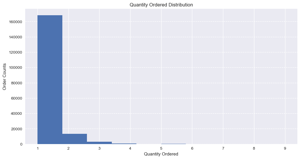
1. Quantity Ordered Distribution
plt.figure(figsize=(12, 6))
plt.hist(df_featured['quantity'])
plt.xlabel('Quantity Ordered')
plt.ylabel('Order Counts')
plt.title('Quantity Ordered Distribution')
plt.grid(axis='y', linestyle='--')
plt.show()
Output:
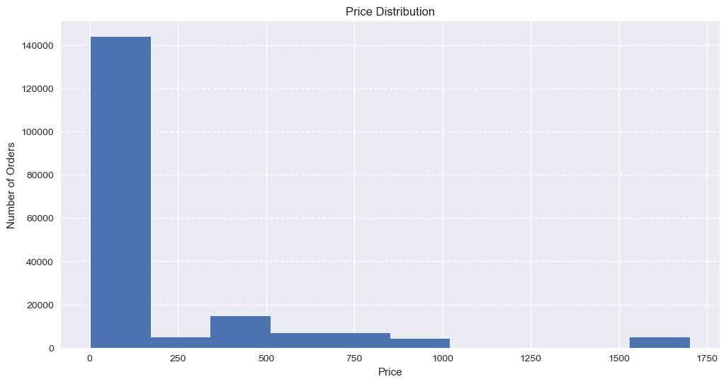
2. Each Price Distribution
plt.figure(figsize=(12, 6))
plt.hist(df_featured['price'])
plt.xlabel('Price')
plt.ylabel('Number of Orders')
plt.title('Price Distribution')
plt.grid(axis='y', linestyle='--')
plt.show()
Output:
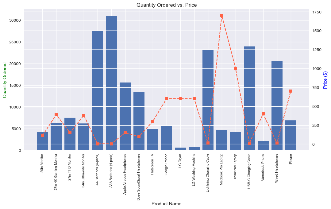
6. Quantity vs Price Analysis
# --- Q5: Quantity vs Price Analysis ---
print("5. Plotting Quantity vs Price...")

# Group data
product_group = df_featured.groupby('product')

quantity = product_group['quantity'].sum()
prices = product_group['price'].mean()
products = [product for product, df_product in product_group]

# Create the figure
fig, ax1 = plt.subplots(figsize=(12, 6))

# Plot Bar Chart (Quantity) on Left Axis
ax2 = ax1.twinx()
ax1.bar(products, quantity) # color='#206fb4', alpha=0.7

# Plot Line Chart (Price) on Right Axis
ax2.plot(products, prices, linestyle='--', marker='s', color='tomato')

# Label Axes
ax1.set_xlabel('Product Name')
ax1.set_ylabel('Quantity Ordered', color='g')
ax2.set_ylabel('Price ($)', color='b')

# FIX: Explicitly set the tick positions before setting labels
ax1.set_xticks(range(len(products)))
ax1.set_xticklabels(products, rotation=90, size=8)

plt.title('Quantity Ordered vs. Price')
plt.show()
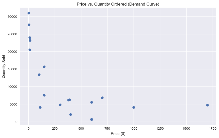
8. Price vs Quantity Ordered
# Price vs Order correlation
# --- Correlation Scatter Plot ---
print("\n6. Plotting Price Elasticity (Scatter)...\n")
product_df = pd.DataFrame({'quantity': quantity, 'price': prices}).reset_index()
print(product_df)

plt.figure(figsize=(10, 6))
plt.scatter(product_df['price'], product_df['quantity'])
# sns.regplot(x='price', y='quantity', data=product_df, logx=True, scatter_kws={"s": 100}, line_kws={"color": "#206fb4"})

plt.title('Price vs. Quantity Ordered (Demand Curve)')
plt.xlabel('Price ($)')
plt.ylabel('Quantity Sold')
plt.grid(True)
plt.show()
Output:
6. Plotting Price Elasticity (Scatter)...

                       product  quantity    price
0                 20in Monitor      4126   109.99
1       27in 4K Gaming Monitor      6239   389.99
2             27in FHD Monitor      7541   149.99
3       34in Ultrawide Monitor      6192   379.99
4        AA Batteries (4-pack)     27615     3.84
5       AAA Batteries (4-pack)     30986     2.99
6     Apple Airpods Headphones     15637   150.00
7   Bose SoundSport Headphones     13430    99.99
8                Flatscreen TV      4813   300.00
9                 Google Phone      5529   600.00
10                    LG Dryer       646   600.00
11          LG Washing Machine       666   600.00
12    Lightning Charging Cable     23169    14.95
13          Macbook Pro Laptop      4725  1700.00
14             ThinkPad Laptop      4128   999.99
15        USB-C Charging Cable     23931    11.95
16             Vareebadd Phone      2068   400.00
17            Wired Headphones     20524    11.99
18                      iPhone      6847   700.00
3. Sales by Month
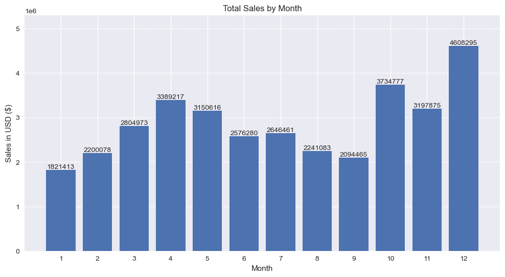
# --- Q1: Sales by Month/monthly sales ---
print("\n1. Plotting Sales by Month...")

monthly_sales = df_featured.groupby('month')['sales'].sum()
print(monthly_sales)

months = range(1, 13)
plt.figure(figsize=(12, 6))
# plt.bar(months, monthly_sales, color='skyblue')

# Add count labels above each bar
bars = plt.bar(months, monthly_sales) # color='#206fb4'
for bar in bars:
    height = bar.get_height()
    plt.text(bar.get_x() + bar.get_width()/2,
             height + 100,  # adjust +100 if needed
             f'{int(height)}', ha='center', va='bottom')

plt.ylim(0, monthly_sales.max() * 1.15) # 1.25 if need extra space

plt.xticks(months)
plt.ylabel('Sales in USD ($)')
plt.xlabel('Month')
plt.title('Total Sales by Month')
plt.grid(axis='y', linestyle='--')
plt.show()
Output:
1. Plotting Sales by Month...
month
1     1821413.16
2     2200078.08
3     2804973.35
4     3389217.98
5     3150616.23
6     2576280.15
7     2646461.32
8     2241083.37
9     2094465.69
10    3734777.86
11    3197875.05
12    4608295.70
Name: sales, dtype: float64
4. Sales by Date
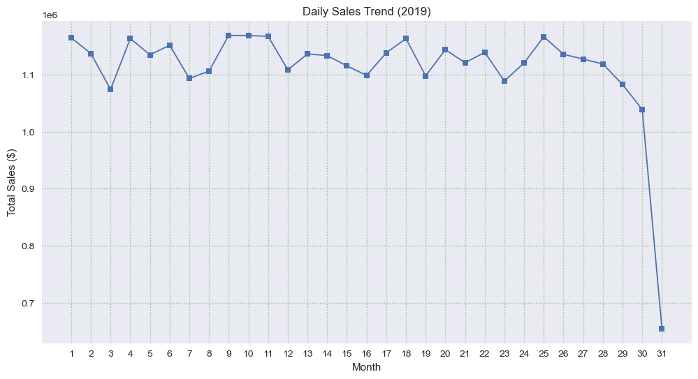
# Sales by Date
monthly_sales = df_featured.groupby('date')['sales'].sum()

print(monthly_sales)

plt.figure(figsize=(12, 6))
# monthly_sales.plot(kind='line', marker='s', linewidth=2, markersize=8)

plt.plot(monthly_sales.index, monthly_sales.values,
         marker='s', linewidth=1.3, markersize=6.2)

# Add numbers near each marker
# for x, y in zip(monthly_sales.index, monthly_sales.values):
#     plt.text(x, y, f"{y:.0f}", fontsize=10, ha='center', va='bottom')

plt.title('Daily Sales Trend (2019)')
plt.xlabel('Month')
plt.ylabel('Total Sales ($)')
plt.grid(axis="both", linestyle=":", alpha=0.4, color="g",)
plt.xticks(range(1, 32))
plt.show()
Output:
fsdfsdfdfsf
5. Sales by Day
# --- Q1: Sales by Day / Daily Sales ---
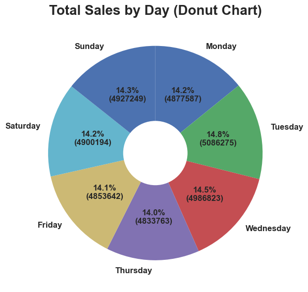
print("\n1. Plotting Sales by Day...")

weekday_order = ['Monday', 'Tuesday', 'Wednesday', 'Thursday', 'Friday', 'Saturday', 'Sunday']
df_featured['day'] = pd.Categorical(df_featured['day'], categories=weekday_order, ordered=True)

# Daily aggregation
daily_sales = df_featured.groupby('day')['sales'].sum().sort_index()
print(daily_sales)


plt.figure(figsize=(12, 6))

# Main pie
wedges, texts, autotexts = plt.pie(
    daily_sales,
    labels=daily_sales.index,
    autopct=lambda pct: f"{pct:.1f}%\n({int(pct/100 * daily_sales.sum())})",
    startangle=90,
    counterclock=False,   # <-- start clockwise
    textprops={'fontsize': 12, 'fontweight': 'bold'}
)

# Create donut hole
centre_circle = plt.Circle((0, 0), 0.30, fc='white')
plt.gca().add_artist(centre_circle)

plt.title("Total Sales by Day (Donut Chart)", fontsize=20, fontweight='bold')
plt.tight_layout()
plt.show()
Output:
1. Plotting Sales by Day...
day
Monday       4877588.21
Tuesday      5086275.40
Wednesday    4986823.36
Thursday     4833763.73
Friday       4853642.26
Saturday     4900195.58
Sunday       4927249.40
Name: sales, dtype: float64
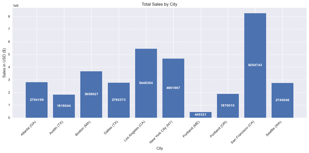
Sales by City
print("2. Plotting Sales by City...")

city_sales = df_featured.groupby('city')['sales'].sum()

# Generate evenly spaced positions
cities = list(city_sales.index)
x_pos = np.arange(len(cities))

plt.figure(figsize=(12, 6))
bars = plt.bar(x_pos, city_sales.values) # Plot bars

# # Add labels above bars
# for bar in bars:
#     height = bar.get_height()
#     plt.text(
#         bar.get_x() + bar.get_width() / 2,
#         height + (height * 0.02),
#         f"{int(height)}",
#         ha="center",
#         va="bottom"
#     )

# Add extra space above tallest bar to avoid cutoff
# plt.ylim(0, city_sales.max() * 1.15) # 1.25 if need extra space

# Add labels above bars
for bar in bars:
    height = bar.get_height()
    plt.text(
        bar.get_x() + bar.get_width() / 2,
        height * 0.5,                 # middle of the bar
        f"{int(height)}",
        ha="center",
        va="center",
        color="white",                # white text looks good inside bars
        fontsize=10,
        fontweight="bold"
    )

# Formatting
plt.xticks(x_pos, cities, rotation=45, ha='right')
plt.ylabel("Sales in USD ($)")
plt.xlabel("City")
plt.title("Total Sales by City")
plt.grid(axis="y", linestyle="--")
plt.tight_layout()
plt.show()
Output:
2. Plotting Sales by City...
4. Orders by Hour
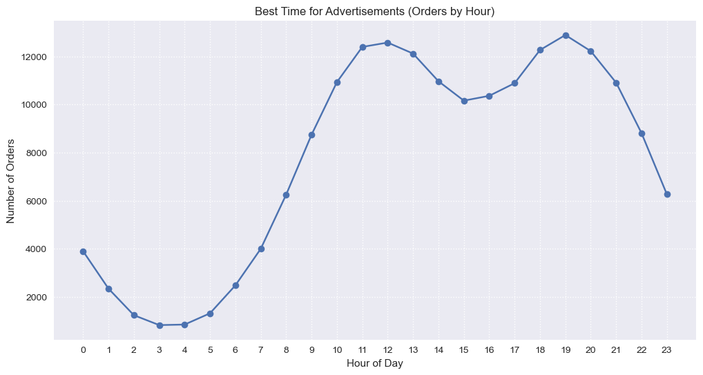
# --- Q3: Orders by Hour ---
print("3. Plotting Orders by Hour...")
hourly_counts = df_featured.groupby(['hour'])['order_id'].count()
hours = [hour for hour, df_hour in df_featured.groupby('hour')]

plt.figure(figsize=(12, 6))
plt.plot(hours, hourly_counts, marker='o') # color='#206fb4'
plt.xticks(hours)
plt.xlabel('Hour of Day')
plt.ylabel('Number of Orders')
plt.title('Best Time for Advertisements (Orders by Hour)')
plt.grid(True, linestyle=':')
plt.show()
Output:
3. Plotting Orders by Hour...
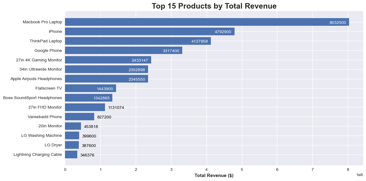
7. Top products by sales/revenue
# Top products by revenue
print("Top 15 Product by sales:\n")

# product_revenue = df_featured.groupby('product')['sales'].sum().sort_values(ascending=False).head(15)
# print(product_revenue)

product_revenue = (
    df_featured.groupby('product')['sales']
    .sum()
    .sort_values(ascending=False)
    .head(15)
)

# # Remove index name and series name
# product_revenue.index.name = None
# product_revenue.name = None

# print(product_revenue.to_string())

# Convert to DataFrame and add serial numbers
df_top = product_revenue.reset_index()
df_top.index = df_top.index + 1   # start index from 1
# df_top.index.name = "S/N"

# Rename columns
df_top.columns = ["Product", "Sales"]

# Print without index name clutter
print(df_top.to_string())

fig, ax = plt.subplots(figsize=(12, 6))
bars = ax.barh(product_revenue.index, product_revenue.values)

# Invert y-axis so largest revenue on top
ax.invert_yaxis()

# Add labels to each bar
for bar in bars:
    width = bar.get_width()
    xpos = width - (product_revenue.max()*0.01)  # slightly inside
    color = 'white' if width > product_revenue.max()*0.15 else 'black'
    ha = 'right' if width > product_revenue.max()*0.15 else 'left'

    ax.text(
        xpos if ha=='right' else width + product_revenue.max()*0.01,
        bar.get_y() + bar.get_height()/2 + 0.1, # y_offset: 0.1
        f'{int(width)}',
        ha=ha,
        va='center',
        fontsize=10,
        # fontweight='bold',
        color=color
    )

# ax.set_yticklabels(product_revenue.index, fontweight='bold') # Make y-axis labels bold

ax.tick_params(axis='y', labelsize=10, labelrotation=0)  # adjust size/rotation if needed
# for label in ax.get_yticklabels():
    # label.set_fontweight('bold')

# for label in ax.get_xticklabels():
    # label.set_fontweight('bold')

ax.set_xlabel('Total Revenue ($)', fontweight='bold')
ax.set_title('Top 15 Products by Total Revenue', fontweight='bold', fontsize=18)

plt.tight_layout()
plt.show()
Output:
Top 15 Product by sales:

                       Product       Sales
1           Macbook Pro Laptop  8032500.00
2                       iPhone  4792900.00
3              ThinkPad Laptop  4127958.72
4                 Google Phone  3317400.00
5       27in 4K Gaming Monitor  2433147.61
6       34in Ultrawide Monitor  2352898.08
7     Apple Airpods Headphones  2345550.00
8                Flatscreen TV  1443900.00
9   Bose SoundSport Headphones  1342865.70
10            27in FHD Monitor  1131074.59
11             Vareebadd Phone   827200.00
12                20in Monitor   453818.74
13          LG Washing Machine   399600.00
14                    LG Dryer   387600.00
15    Lightning Charging Cable   346376.55
5. Products Sold Together
# --- Q4: Products Sold Together ---
print("4. Calculating Products Sold Together...\n")

# Find duplicate Order IDs (items in same cart)
df_dup = df_featured[df_featured['order_id'].duplicated(keep=False)].copy()
df_dup['grouped'] = df_dup.groupby('order_id')['product'].transform(lambda x: ','.join(x))
df_dup = df_dup[['order_id', 'grouped']].drop_duplicates()

# Count pairs
count = Counter()
for row in df_dup['grouped']:
    row_list = row.split(',')
    count.update(Counter(combinations(row_list, 2)))

print("Top 10 Most Common Pairs:")
i = 1
for pair, freq in count.most_common(10):
    print(f"{i}. {pair}: {freq}")
    i+= 1
Output:
4. Calculating Products Sold Together...

Top 10 Most Common Pairs:
1. ('iPhone', 'Lightning Charging Cable'): 1002
2. ('Google Phone', 'USB-C Charging Cable'): 985
3. ('iPhone', 'Wired Headphones'): 447
4. ('Google Phone', 'Wired Headphones'): 413
5. ('Vareebadd Phone', 'USB-C Charging Cable'): 361
6. ('iPhone', 'Apple Airpods Headphones'): 360
7. ('Google Phone', 'Bose SoundSport Headphones'): 220
8. ('USB-C Charging Cable', 'Wired Headphones'): 159
9. ('Vareebadd Phone', 'Wired Headphones'): 143
10. ('Lightning Charging Cable', 'Wired Headphones'): 92
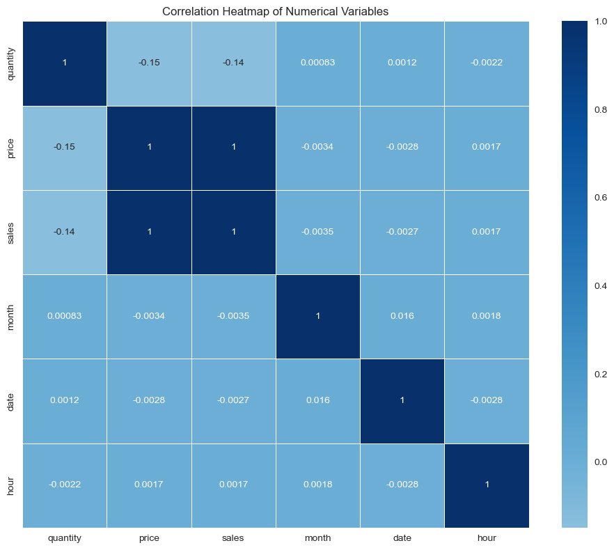
Correlation between numeric fields
# Correlation heatmap
# numerical_cols = ['quantity_ordered', 'price_each', 'sales', 'month', 'day', 'hour']
numerical_cols = ['quantity', 'price', 'sales', 'month', 'date', 'hour']
correlation_matrix = df_featured[numerical_cols].corr()

plt.figure(figsize=(10, 8))
# sns.color_palette("seagreen", as_cmap=True)
sns.color_palette("Blues", as_cmap=True)
# sns.heatmap(correlation_matrix, annot=True, cmap='coolwarm', center=0,
sns.heatmap(correlation_matrix, annot=True, cmap='Blues', center=0,
           square=True, linewidths=0.5)
plt.title('Correlation Heatmap of Numerical Variables')
plt.tight_layout()
plt.show()