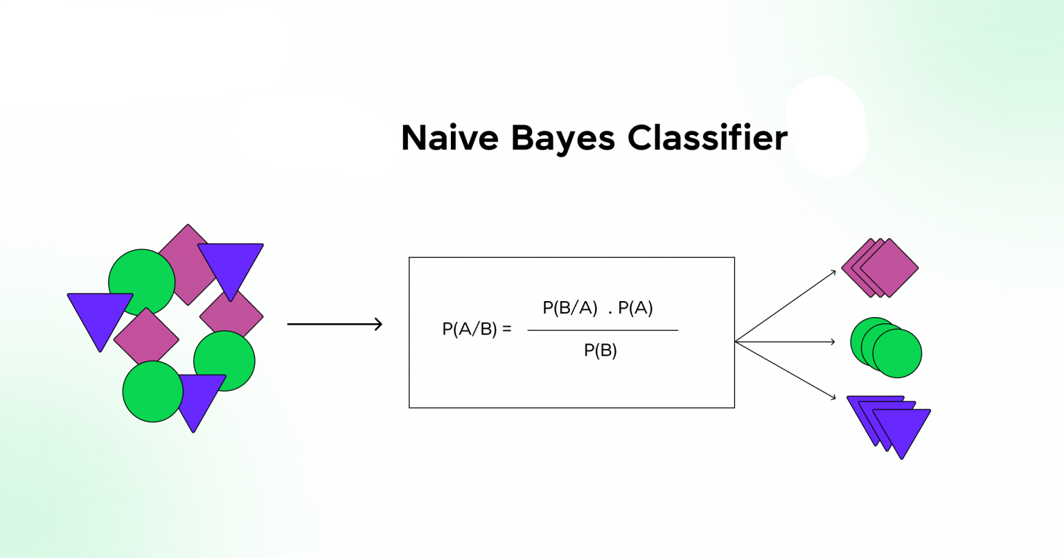
Naive Bayes Classifier
(A Complete Guide with Example and Python Code)
1. Introduction
Machine Learning allows computers to learn patterns from data and make decisions without being explicitly programmed. One of the most popular and simple algorithms used for classification problems is the Naive Bayes Algorithm.
Naive Bayes is widely used in:
- Spam email detection
- Sentiment analysis
- Document classification
- Medical diagnosis
Despite its simplicity, it performs surprisingly well, especially for text-based problems.
2. What is Naive Bayes Algorithm?
Naive Bayes is a supervised learning algorithm based on Bayes’ Theorem. It predicts the class of a data point by calculating probabilities and choosing the class with the highest probability.
It is called “Naive” because it assumes that all features are independent of each other, which is usually not true in real life.
3. Bayes’ Theorem
Bayes’ Theorem describes the probability of an event based on prior knowledge.
Formula:
\(P(A|B) = \frac{P(B|A),P(A)}{P(B)}\)
Explanation:
- (P(A)) → Prior probability
-
(P(B A)) → Likelihood -
(P(A B)) → Posterior probability - (P(B)) → Evidence
In classification, we calculate the posterior probability for each class and select the maximum.
4. How Naive Bayes Works
For a data point with features (x_1, x_2, …, x_n):
\[P(c|x_1,x_2,...,x_n) \propto P(c)\prod_{i=1}^{n} P(x_i|c)\]- (P(c)) → Probability of class
-
(P(x_i c)) → Probability of feature given class
The denominator is ignored because it is the same for all classes.
5. Types of Naive Bayes
5.1 Gaussian Naive Bayes
- Used for continuous data
- Assumes features follow a normal distribution
5.2 Multinomial Naive Bayes
- Used for text data
- Based on word frequency
- Common in spam filtering
5.3 Bernoulli Naive Bayes
- Binary features (0 or 1)
- Checks presence/absence of features
6. Manual Numerical Example (Spam Detection)
Dataset (10 Emails)
| Text | Class | |
|---|---|---|
| E1 | win money | Spam |
| E2 | win prize | Spam |
| E3 | claim prize now | Spam |
| E4 | win cash offer | Spam |
| E5 | free money win | Spam |
| E6 | meeting today | Not Spam |
| E7 | project meeting | Not Spam |
| E8 | team meeting today | Not Spam |
| E9 | project deadline | Not Spam |
| E10 | schedule meeting | Not Spam |
Step 1: Vocabulary
\(V = {win, money, prize, claim, now, cash, offer, free, meeting, today, project, team, deadline, schedule}\)
Vocabulary size: \(|V| = 14\)
Step 2: Prior Probabilities
Total emails = 10
\[P(Spam) = \frac{5}{10} = 0.5\] \[P(Not\ Spam) = \frac{5}{10} = 0.5\]Step 3: Word Frequencies
Spam Emails (Total words = 13)
| Word | Count |
|---|---|
| win | 3 |
| money | 2 |
| prize | 2 |
| claim | 1 |
| now | 1 |
| cash | 1 |
| offer | 1 |
| free | 1 |
Not Spam Emails (Total words = 12)
| Word | Count |
|---|---|
| meeting | 4 |
| today | 2 |
| project | 2 |
| team | 1 |
| deadline | 1 |
| schedule | 1 |
| (others) | 0 |
Step 4: Laplace Smoothing Formula
\[P(word|class) = \frac{count + 1}{total\ words + |V|}\]- Spam denominator = (13 + 14 = 27)
- Not Spam denominator = (12 + 14 = 26)
Predictions
Prediction 1: Equal Probabilities
Email: "win meeting"
Spam Probability
\[P(Spam) \times P(win|Spam) \times P(meeting|Spam)\] \[= 0.5 \times \frac{3+1}{27} \times \frac{0+1}{27}\] \[= 0.5 \times \frac{4}{27} \times \frac{1}{27} = 0.0027\]Not Spam Probability
\[0.5 \times \frac{0+1}{26} \times \frac{4+1}{26}\] \[= 0.5 \times \frac{1}{26} \times \frac{5}{26} = 0.0027\]Decision:
Equal probabilities
Prediction 2: Spam Email
Email: "claim free prize now"
Words in the email:
- claim
- free
- prize
- now
Spam Probability
Using Laplace smoothing (Spam denominator = 27, since total spam words = 13 and |V| = 14)
Counts from Spam class:
- claim = 1
- free = 1
- prize = 2
- now = 1
Not Spam Probability
Using Laplace smoothing (Not Spam denominator = 26, since total not-spam words = 12 and |V| = 14)
Counts from Not Spam class:
- claim = 0
- free = 0
- prize = 0
- now = 0
Decision
\[P(Spam|Email) > P(NotSpam|Email)\]Classified as Spam
Prediction 3: Not Spam Email
Email: "project meeting today"
Spam Probability
\[0.5 \times \frac{0+1}{27} \times \frac{0+1}{27} \times \frac{0+1}{27}\] \[= 0.5 \times \frac{1}{27^3} = 0.000025\]Not Spam Probability
\[0.5 \times \frac{2+1}{26} \times \frac{4+1}{26} \times \frac{2+1}{26}\] \[= 0.5 \times \frac{3}{26} \times \frac{5}{26} \times \frac{3}{26} = 0.00399\]Decision:
Classified as Not Spam
Prediction 4: Zero Probability Problem (Without Laplace)
Email: "deadline schedule"
Without Laplace Smoothing
Spam:
- deadline = 0
- schedule = 0
Not Spam:
- deadline = 1
- schedule = 1
Spam probability becomes zero → model breaks
Fix Using Laplace Smoothing
Spam Probability
\(0.5 \times \frac{0+1}{27} \times \frac{0+1}{27} = 0.00068\)
Not Spam Probability
\[0.5 \times \frac{1+1}{26} \times \frac{1+1}{26} = 0.00147\]Decision:
Classified as Not Spam
Key Takeaways
- Naive Bayes uses probability multiplication
- One unseen word → probability becomes zero
- Laplace smoothing fixes this issue
- Works extremely well for text classification
10. Python Implementation (Scikit-Learn)
# 1. Import required libraries
import pandas as pd
from sklearn.feature_extraction.text import CountVectorizer
from sklearn.naive_bayes import MultinomialNB

# 2. Training Dataset (Same as Manual Example)
emails = [
    "win money",
    "win prize",
    "claim prize now",
    "win cash offer",
    "free money win",
    "meeting today",
    "project meeting",
    "team meeting today",
    "project deadline",
    "schedule meeting"
]

labels = [
    "Spam",
    "Spam",
    "Spam",
    "Spam",
    "Spam",
    "Not Spam",
    "Not Spam",
    "Not Spam",
    "Not Spam",
    "Not Spam"
]

# 3. Convert Text to Feature Vectors (Bag of Words)
vectorizer = CountVectorizer()
X = vectorizer.fit_transform(emails)

# # Check vocabulary (optionl)
# print("Vocabulary:")
# print(vectorizer.vocabulary_)
# print("Vocabulary size:", len(vectorizer.vocabulary_))

# Train Multinomial Naive Bayes Model
# (Laplace smoothing is ON by default → alpha=1)
model = MultinomialNB(alpha=1)
model.fit(X, labels)

test_emails = [
    "win meeting",
    "claim free prize now",
    "project meeting today",
    "deadline schedule"
]

X_test = vectorizer.transform(test_emails)

predictions = model.predict(X_test)
probabilities = model.predict_proba(X_test)

for email, pred, prob in zip(test_emails, predictions, probabilities):
    print("\nEmail:", email)
    print("Prediction:", pred)
    print("Class probabilities:", prob)
Output:
Email: win meeting
Prediction: Not Spam
Class probabilities: [0.53840473 0.46159527]

Email: claim free prize now
Prediction: Spam
Class probabilities: [0.05364601 0.94635399]

Email: project meeting today
Prediction: Not Spam
Class probabilities: [0.98266508 0.01733492]

Email: deadline schedule
Prediction: Not Spam
Class probabilities: [0.82349619 0.17650381]
import pandas as pd
from sklearn.preprocessing import LabelEncoder
from sklearn.naive_bayes import GaussianNB

import warnings
warnings.filterwarnings("ignore")

# Dataset
data = {
    'Outlook': ['Sunny','Sunny','Overcast','Rain','Rain','Rain','Overcast','Sunny','Sunny','Rain','Sunny','Overcast','Overcast','Rain'],
    'Temperature': ['Hot','Hot','Hot','Mild','Cool','Cool','Cool','Mild','Cool','Mild','Mild','Mild','Hot','Mild'],
    'Humidity': ['High','High','High','High','Normal','Normal','Normal','High','Normal','Normal','Normal','High','Normal','High'],
    'Wind': ['Weak','Strong','Weak','Weak','Weak','Strong','Strong','Weak','Weak','Weak','Strong','Strong','Weak','Strong'],
    'PlayTennis': ['No','No','Yes','Yes','Yes','No','Yes','No','Yes','Yes','Yes','Yes','Yes','No']
}
df = pd.DataFrame(data)

# Label encode features
X = df[['Outlook','Temperature','Humidity','Wind']]
y = df['PlayTennis'].map({'No':0,'Yes':1})

label_encoders = {}
for col in X.columns:
    le = LabelEncoder()
    X[col] = le.fit_transform(X[col])
    label_encoders[col] = le

# Train GaussianNB
gnb = GaussianNB()
gnb.fit(X, y)

# 5 inputs to predict
original_inputs = [
    {'Outlook':'Sunny','Temperature':'Hot','Humidity':'High','Wind':'Weak'},
    {'Outlook':'Rain','Temperature':'Mild','Humidity':'Normal','Wind':'Weak'},
    {'Outlook':'Overcast','Temperature':'Hot','Humidity':'High','Wind':'Weak'},
    {'Outlook':'Sunny','Temperature':'Cool','Humidity':'Normal','Wind':'Strong'},
    {'Outlook':'Rain','Temperature':'Cool','Humidity':'High','Wind':'Strong'}
]

input_data = pd.DataFrame(original_inputs)

# Encode inputs
for col in input_data.columns:
    input_data[col] = label_encoders[col].transform(input_data[col])

# Predict probabilities and classes
probs = gnb.predict_proba(input_data)
preds = gnb.predict(input_data)

# Display in requested format
for i in range(len(input_data)):
    feat = original_inputs[i]
    print(f"\nPrediction {i+1}:")
    print(feat)
    print(f"P(No|{feat['Outlook']}, {feat['Temperature']}, {feat['Humidity']}, {feat['Wind']})  = {probs[i][0]:.4f}")
    print(f"P(Yes|{feat['Outlook']}, {feat['Temperature']}, {feat['Humidity']}, {feat['Wind']}) = {probs[i][1]:.4f}")
    print("Predicted PlayTennis:", "No" if preds[i]==0 else "Yes")
Output:
Prediction 1:
{'Outlook': 'Sunny', 'Temperature': 'Hot', 'Humidity': 'High', 'Wind': 'Weak'}
P(No|Sunny, Hot, High, Weak)  = 0.8007
P(Yes|Sunny, Hot, High, Weak) = 0.1993
Predicted PlayTennis: No

Prediction 2:
{'Outlook': 'Rain', 'Temperature': 'Mild', 'Humidity': 'Normal', 'Wind': 'Weak'}
P(No|Rain, Mild, Normal, Weak)  = 0.0547
P(Yes|Rain, Mild, Normal, Weak) = 0.9453
Predicted PlayTennis: Yes

Prediction 3:
{'Outlook': 'Overcast', 'Temperature': 'Hot', 'Humidity': 'High', 'Wind': 'Weak'}
P(No|Overcast, Hot, High, Weak)  = 0.0130
P(Yes|Overcast, Hot, High, Weak) = 0.9870
Predicted PlayTennis: Yes

Prediction 4:
{'Outlook': 'Sunny', 'Temperature': 'Cool', 'Humidity': 'Normal', 'Wind': 'Strong'}
P(No|Sunny, Cool, Normal, Strong)  = 0.3730
P(Yes|Sunny, Cool, Normal, Strong) = 0.6270
Predicted PlayTennis: Yes

Prediction 5:
{'Outlook': 'Rain', 'Temperature': 'Cool', 'Humidity': 'High', 'Wind': 'Strong'}
P(No|Rain, Cool, High, Strong)  = 0.6269
P(Yes|Rain, Cool, High, Strong) = 0.3731
Predicted PlayTennis: No
8. Advantages of Naive Bayes
- Simple and fast
- Works well with high-dimensional data
- Requires less training data
- Excellent for text classification
- Easy to interpret
9. Limitations of Naive Bayes
- Assumes feature independence
- Performs poorly if features are correlated
- Probability estimates may be inaccurate
- Sensitive to input data quality
11. Evaluation Metrics
- Accuracy
- Precision
- Recall
- F1-score
- Confusion Matrix
These metrics help measure model performance.
12. Applications of Naive Bayes
- Spam filtering
- Sentiment analysis
- News categorization
- Medical diagnosis
- Recommendation systems
13. Conclusion
Naive Bayes is a powerful yet simple classification algorithm based on probability theory. Although it makes strong assumptions, it performs exceptionally well in many real-world applications, especially text classification.
Its simplicity, speed, and effectiveness make it a must-learn algorithm for beginners in Machine Learning.