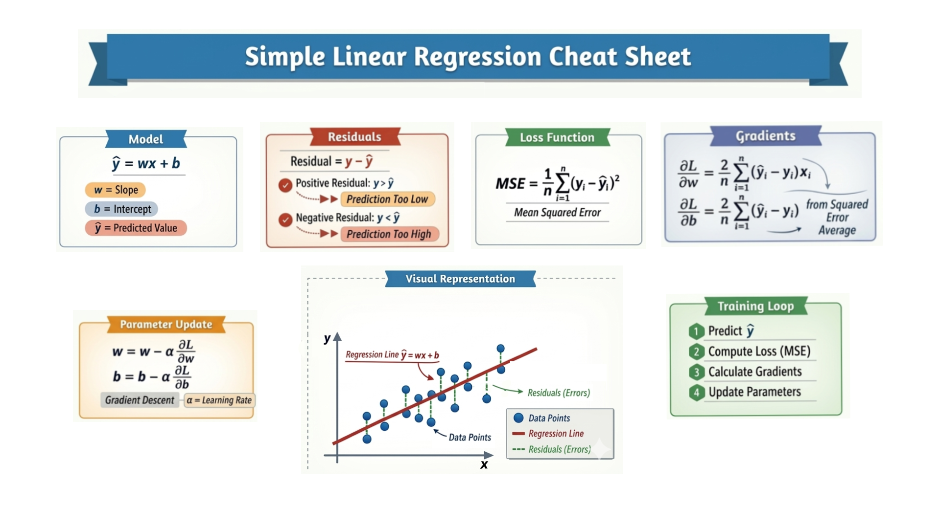
Here are the major steps to implement Simple Linear Regression from scratch.

1. Prepare the Dataset

You start with input–output data.

X → independent variable (feature)
y → dependent variable (target)

The goal of the model is to learn the relationship between X and y so that it can predict the target value for new inputs.

2. Define the Model (Linear Equation)

Simple linear regression assumes a straight-line relationship between the input and output:

\[\hat{y} = wx + b\]

Where:

w → weight (slope of the line)
b → bias (intercept)
x → input feature
ŷ → predicted value

Intuition:

w (slope) controls how steep the line is.
b (intercept) shifts the line up or down.
The algorithm adjusts the line so that it passes as close as possible to all data points.

Visually:

Data → scattered points
Model → straight line
Training → moving the line until it fits the points best

3. Initialize Parameters

Before training begins, we start with initial parameter values:

w = 0
b = 0
α = 0.01  # learning rate

Where:

w → weight
b → bias
α → learning rate (controls how large each update step is)

4. Make Predictions

Using the model equation, we compute predictions for each input:

\[\hat{y} = wx + b\]

This gives the predicted output for every data point.

5. Understand Residuals

A residual is the difference between the actual value and predicted value:

\[\text{Residual} = y - \hat{y}\]

Residuals tell us how wrong each prediction is:

Positive residual → prediction too small
Negative residual → prediction too large

6. Calculate the Loss (Error)

We measure how far the predictions are from the true values using Mean Squared Error (MSE):

\[MSE = \frac{1}{n}\sum_{i=1}^{n}(y_i - \hat{y}_i)^2\]

Where:

n = number of samples
yᵢ = actual value
ŷᵢ = predicted value

The goal of training is to find values of w and b that minimize this loss, i.e., make residuals as small as possible.

7. Compute Gradients (Derivatives)

To reduce the loss, we calculate how sensitive the loss is to changes in the parameters.

Gradients show how the parameters should change to reduce the loss.

\[\frac{\partial L}{\partial w} = \frac{2}{n}\sum_{i=1}^{n}(\hat{y}_i - y_i)x_i\] \[\frac{\partial L}{\partial b} = \frac{2}{n}\sum_{i=1}^{n}(\hat{y}_i - y_i)\]

Why 2/n?

The MSE is \((\frac{1}{n}\sum (y_i - \hat{y}_i)^2)\)
Differentiating \(((y_i - \hat{y}_i)^2)\) gives \(2*(ŷ - y)\)
Multiply by \(1/n\) from the mean → \(2/n\)

This scaling ensures the gradient points in the correct direction and is proportional to the average error.

8. Update Parameters (Gradient Descent)

We update the parameters in the opposite direction of the gradients:

\[w = w - \alpha \frac{\partial L}{\partial w}\] \[b = b - \alpha \frac{\partial L}{\partial b}\]

Intuition:

If prediction > actual → gradient pushes line downward
If prediction < actual → gradient pushes line upward

The learning rate α controls how big each adjustment is.

9. Repeat for Many Iterations

Each full pass through the dataset is called an epoch.

During each epoch:

Predict values
Compute loss
Compute gradients
Update parameters

Repeat for many epochs until the loss converges (stops decreasing significantly).

10. Use the Model for Prediction

After training is complete, the model has learned the optimal w and b.

For any new input x:

\[\hat{y} = wx + b\]

This allows the model to estimate target values for unseen data.

Final Algorithm (Summary)

Load dataset \((X, y)\)
Initialize w, b, and learning rate
Loop for a number of epochs
Compute predictions
Compute residuals and loss (MSE)
Compute gradients
Update parameters using gradient descent
Repeat until loss converges
Use the trained model for predictions

Linear Regression from Scratch: 5 Iterations of Gradient

Iteration 1

1. Dataset

We have 5 data points:

\[X = [1, \enspace 2, \enspace 3, \enspace 4, \enspace 5], \quad y = [3, \enspace 5, \enspace 7, \enspace 9, \enspace 11]\]

We start with initial parameters:

\[w = 0, \quad b = 0\]

2. Making Predictions

The predicted values \((\hat{y})\) are calculated using the linear model:

\[\hat{y} = w \cdot X + b\]

Substituting \((w=0, b=0)\):

\[\hat{y} = [0\cdot1 + 0, \enspace 0\cdot2 + 0, \enspace 0\cdot3 + 0, \enspace 0\cdot4 + 0, \enspace 0\cdot5 + 0] = [0, 0, 0, 0, 0]\]

At this stage, our model predicts all zeros because both weight and bias are zero.

3. Calculating Errors

The error for each data point is:

\[\text{Error} = y - \hat{y}\] \[= [3, 5, 7, 9, 11] - [0, 0, 0, 0, 0] = [3, 5, 7, 9, 11]\]

This shows how far off our predictions are from the actual values.

4. Calculating Loss (Mean Squared Error)

We use Mean Squared Error (MSE):

\[J(w, b) = \frac{1}{n} \sum_{i=1}^{n} (\hat{y}_i - y_i)^2\] \[= \frac{1}{5} [(-3)^2 + (-5)^2 + (-7)^2 + (-9)^2 + (-11)^2]\] \[= \frac{1}{5} [9 + 25 + 49 + 81 + 121] = \frac{285}{5} = 57\]

This is the “cost” of our model with the current parameters.

5. Calculating Gradients

We compute partial derivatives to know the direction in which to adjust parameters.

A. Gradient w.r.t Weight (w)

\[\frac{\partial J}{\partial w} = \frac{2}{n} \sum_{i=1}^{n} (\hat{y}_i - y_i) x_i\] \[d_w = \frac{2}{5} [(-3\cdot1) + (-5\cdot2) + (-7\cdot3) + (-9\cdot4) + (-11\cdot5)] = \frac{2}{5}(-125) = -50\]

Step by step:

\[(-3\cdot1) + (-5\cdot2) + (-7\cdot3) + (-9\cdot4) + (-11\cdot5) = -3 - 10 - 21 - 36 - 55 = -125\] \[d_w = \frac{2}{5}(-125) = -50\]

Negative gradient → we need to increase (w) to reduce loss.

B. Gradient w.r.t Bias (b)

\[\frac{\partial J}{\partial b} = \frac{2}{n} \sum_{i=1}^{n} (\hat{y}_i - y_i)\] \[d_b = \frac{2}{5} [(-3) + (-5) + (-7) + (-9) + (-11)] = \frac{2}{5}(-35) = -14\]

Step by step:

\[(-3) + (-5) + (-7) + (-9) + (-11) = -35\] \[d_b = \frac{2}{5}(-35) = -14\]

Negative gradient → we also need to increase (b) to reduce loss.

6. Updating Parameters

Using gradient descent with learning rate \((\eta = 0.01)\):

\[w = w - \eta \cdot d_w = 0 - 0.01(-50) = 0.5\] \[b = b - \eta \cdot d_b = 0 - 0.01(-14) = 0.14\]

After one iteration, the model has learned a little: weight (w = 0.5) and bias (b = 0.14).

Iteration 2

1. Making Predictions

Using updated parameters from Iteration 1:

\[w = 0.5\] \[b = 0.14\]

Using the linear model:

\[\hat{y} = w \cdot X + b\]

Substituting \((w = 0.5, b = 0.14)\):

\[\hat{y} = [0.5\cdot 1 + 0.14, \enspace 0.5\cdot 2 + 0.14, \enspace 0.5\cdot 3 + 0.14, \enspace 0.5\cdot 4 + 0.14, \enspace 0.5\cdot 5 + 0.14]\] \[= [0.5 + 0.14, \enspace 1.0 + 0.14, \enspace 1.5 + 0.14, \enspace 2.0 + 0.14, \enspace 2.5 + 0.14]\] \[= [0.64, \enspace 1.14, \enspace 1.64, \enspace 2.14, \enspace 2.64]\]

The predictions are now slightly closer to the true values, but still far away.

2. Calculating Errors

\[\text{Error} = \hat{y} - y\] \[= [0.64 - 3, \enspace 1.14 - 5, \enspace 1.64 - 7, \enspace 2.14 - 9, \enspace 2.64 - 11]\] \[= [-2.36, -3.86, -5.36, -6.86, -8.36]\]

3. Calculating Loss (MSE)

\[J(w, b) = \frac{1}{5} \sum (\hat{y}_i - y_i)^2\] \[= \frac{1}{5} [(-2.36)^2 + (-3.86)^2 + (-5.36)^2 + (-6.86)^2 + (-8.36)^2]\] \[= \frac{1}{5} [5.5696+ 14.8996 + 28.7296 + 47.0596 + 69.8896]\] \[= \frac{1}{5} [166.148]\] \[= 33.2296 \approx 33.23\]

Loss has decreased from 57 → 33.23. The model is learning.

4. Calculating Gradients

A. Gradient w.r.t Weight (w)

\[\frac{\partial J}{\partial w}/d_w = \frac{2}{n} \sum_{i=1}^{n} (\hat{y}_i - y_i) x_i\] \[d_w = \frac{2}{5} [(-2.36 \cdot 1) + (-3.86 \cdot 2) + (-5.36 \cdot 3) + (-6.86 \cdot 4) + (-8.36 \cdot 5)]\] \[= \frac{2}{5}(-2.36 - 7.72 - 16.08 - 27.44 - 41.8)\] \[= \frac{2}{5}(-95.4)\] \[= -38.16\]

B. Gradient w.r.t Bias (b)

\[\frac{\partial J}{\partial b}/d_b = \frac{2}{n} \sum_{i=1}^{n} (\hat{y}_i - y_i)\] \[= \frac{2}{5} [(-2.36) + (-3.86) + (-5.36) + (-6.86) + (-8.36)]\] \[= \frac{2}{5} [-2.36 - 3.86 - 5.36 - 6.86 - 8.36]\] \[= \frac{2}{5}(-26.8)\] \[= -10.72\]

5. Updating Parameters

\((\eta = 0.01)\)

\[w = w - \eta \cdot d_w\] \[= 0.5 - 0.01(-38.16)\] \[= 0.5 + 0.3816\] \[= 0.8816\] \[b = b - \eta \cdot d_b\] \[= 0.14 - 0.01(-10.72)\] \[= 0.14 + 0.1072\] \[= 0.2472\]

After iteration 2: \((w = 0.8816, b = 0.2472)\)

Iteration 3

1. Making Predictions

Using updated parameters from Iteration 2:

\[w = 0.8816\] \[b = 0.2472\]

Using the linear model:

\[\hat{y} = w \cdot X + b\]

Substituting \((w = 0.8816, b = 0.2472)\):

\[\hat{y} = [0.8816\cdot 1 + 0.2472, \enspace 0.8816\cdot 2 + 0.2472, \enspace 0.8816\cdot 3 + 0.2472, \enspace 0.8816\cdot 4 + 0.2472, \enspace 0.8816\cdot 5 + 0.2472]\] \[= [0.8816 + 0.2472, \enspace 1.7632 + 0.2472, \enspace 2.6448 + 0.2472, \enspace 3.5264 + 0.2472, \enspace 4.408 + 0.2472]\]

\(= [1.1288, \enspace 2.0104, \enspace 2.892, \enspace 3.7736, \enspace 4.6552]\) \(= [1.1288, \enspace 2.0104, \enspace 2.892, \enspace 3.7736, \enspace 4.6552]\)

The predictions continue moving closer to the actual values.

2. Calculating Errors

\[\text{Error} = \hat{y} - y\] \[= [1.1288 - 3, \enspace 2.0104 - 5, \enspace 2.892 - 7, \enspace 3.7736 - 9, \enspace 4.6552 - 11]\] \[= [-1.8712, -2.9896, -4.108, -5.2264, -6.3448]\]

3. Calculating Loss (MSE)

\[J(w, b) = \frac{1}{5} \sum (\hat{y}_i - y_i)^2\] \[= \frac{1}{5} [(-1.8712)^2 + (-2.9896)^2 + (-4.108)^2 + (-5.2264)^2 + (-6.3448)^2]\] \[= \frac{1}{5} [3.50138944 + 8.93770816 + 16.875664 + 27.31424896 + 40.25447104]\] \[= \frac{1}{5} [96.8834816] = 19.37669632 \approx 19.38\]

Loss has decreased further, showing the model is improving.

4. Calculating Gradients

A. Gradient w.r.t Weight (w)

\[\frac{\partial J}{\partial w}/d_w = \frac{2}{n} \sum_{i=1}^{n} (\hat{y}_i - y_i) x_i\] \[d_w = \frac{2}{5} [(-1.8712 \cdot 1) + (-2.9896 \cdot 2) + (-4.108 \cdot 3) + (-5.2264 \cdot 4) + (-6.3448 \cdot 5)]\] \[= \frac{2}{5}(-1.8712 - 5.9792 - 12.324 - 20.9056 - 31.724)\] \[= \frac{2}{5}(-72.804) = -29.1216\]

B. Gradient w.r.t Bias (b)

\[\frac{\partial J}{\partial b}/d_b = \frac{2}{n} \sum_{i=1}^{n} (\hat{y}_i - y_i)\] \[d_b = \frac{2}{5} [(-1.8712) + (-2.9896) + (-4.108) + (-5.2264) + (-6.3448)]\] \[= \frac{2}{5}(-20.54) = -8.216\]

5. Updating Parameters

\[(\eta = 0.01)\] \[w = w - \eta \cdot d_w\] \[= 0.8816 - 0.01(-29.1216)\] \[= 0.8816 + 0.291216\] \[= 1.172816\] \[b = b - \eta \cdot d_b\] \[= 0.2472 - 0.01(-8.216)\] \[= 0.2472 + 0.08216\] \[= 0.32936\]

After iteration 3: \((w = 1.172816, b = 0.32936)\)

Iteration 4

1. Making Predictions

Using updated parameters from Iteration 3:

\[w = 1.172816\] \[b = 0.32936\]

Using the linear model:

\[\hat{y} = w \cdot X + b\]

Substituting \((w = 1.172816, b = 0.32936)\):

\[\hat{y} = [1.172816\cdot 1 + 0.32936, \enspace 1.172816\cdot 2 + 0.32936, \enspace 1.172816\cdot 3 + 0.32936, \enspace 1.172816\cdot 4 + 0.32936, \enspace 1.172816\cdot 5 + 0.32936]\] \[= [1.172816 + 0.32936, \enspace 2.345632 + 0.32936, \enspace 3.518448 + 0.32936, \enspace 4.691264 + 0.32936, \enspace 5.86408 + 0.32936]\] \[= [1.502176, \enspace 2.674992, \enspace 3.847808, \enspace 5.020624, \enspace 6.19344]\]

The predictions continue to move closer to the actual values.

2. Calculating Errors

\[\text{Error} = \hat{y} - y\] \[= [1.502176 - 3, \enspace 2.674992 - 5, \enspace 3.847808 - 7, \enspace 5.020624 - 9, \enspace 6.19344 - 11]\] \[= [-1.497824, -2.325008, -3.152192, -3.979376, -4.80656]\]

3. Calculating Loss (MSE)

\[J(w, b) = \frac{1}{5} \sum (\hat{y}_i - y_i)^2\] \[= \frac{1}{5} [(-1.497824)^2 + (-2.325008)^2 + (-3.152192)^2 + (-3.979376)^2 + (-4.80656)^2]\] \[= \frac{1}{5} [2.24347671 + 5.4056622 + 9.93631439 + 15.83543328 + 23.10301879]\] \[= \frac{1}{5} [56.52390537]\] \[= 11.30478107 \approx 11.30\]

Loss continues decreasing, indicating the model is learning the correct relationship.

4. Calculating Gradients

A. Gradient w.r.t Weight (w)

\[\frac{\partial J}{\partial w}/d_w = \frac{2}{n} \sum_{i=1}^{n} (\hat{y}_i - y_i) x_i\] \[d_w = \frac{2}{5} [(-1.497824 \cdot 1) + (-2.325008 \cdot 2) + (-3.152192 \cdot 3) + (-3.979376 \cdot 4) + (-4.80656 \cdot 5)]\] \[= \frac{2}{5}(-1.497824 - 4.650016 - 9.456576 - 15.917504 - 24.0328)\] \[= \frac{2}{5}(-55.55472)\] \[= -22.221888\]

B. Gradient w.r.t Bias (b)

\[\frac{\partial J}{\partial b}/d_b = \frac{2}{n} \sum_{i=1}^{n} (\hat{y}_i - y_i)\] \[d_b = \frac{2}{5} [(-1.497824) + (-2.325008) + (-3.152192) + (-3.979376) + (-4.80656)]\] \[= \frac{2}{5}(-15.761)\] \[= -6.304384\]

5. Updating Parameters

\[(\eta = 0.01)\] \[w = w - \eta \cdot d_w\] \[= 1.172816 - 0.01(-22.221888)\] \[= 1.172816 + 0.22221888\] \[= 1.39503488\] \[b = b - \eta \cdot d_b\] \[= 0.32936 - 0.01(-6.304384)\] \[= 0.32936 + 0.06304384\] \[= 0.39240384\]

After iteration 4: \((w = 1.39503488, b = 0.39240384)\)

Iteration 5

1. Making Predictions

Using updated parameters from Iteration 4:

\[w = 1.39503488\] \[b = 0.39240384\]

Using the linear model:

\[\hat{y} = w \cdot X + b\]

Substituting \((w = 1.39503488, b = 0.39240384)\):

\[\hat{y} = [1.39503488\cdot 1 + 0.39240384, \enspace 1.39503488\cdot 2 + 0.39240384, \enspace 1.39503488\cdot 3 + 0.39240384, \enspace 1.39503488\cdot 4 + 0.39240384, \enspace 1.39503488\cdot 5 + 0.39240384]\] \[= [1.39503488 + 0.39240384, \enspace 2.79006976 + 0.39240384, \enspace 4.18510464 + 0.39240384, \enspace 5.58013952 + 0.39240384, \enspace 6.9751744 + 0.39240384]\] \[= [1.78743872, \enspace 3.1824736, \enspace 4.57750848, \enspace 5.97254336, \enspace 7.36757824]\]

The predictions are getting closer to the true values.

2. Calculating Errors

\[\text{Error} = \hat{y} - y\] \[= [1.78743872 - 3, \enspace 3.1824736 - 5, \enspace 4.57750848 - 7, \enspace 5.97254336 - 9, \enspace 7.36757824 - 11]\] \[= [-1.21256128, -1.8175264, -2.42249152, -3.02745664, -3.63242176]\]

3. Calculating Loss (MSE)

\[J(w, b) = \frac{1}{5} \sum (\hat{y}_i - y_i)^2\] \[= \frac{1}{5} [(-1.21256128)^2 + (-1.8175264)^2 + (-2.42249152)^2 + (-3.02745664)^2 + (-3.63242176)^2]\] \[= \frac{1}{5} [1.47030504 + 3.30340191 + 5.86846117 + 9.16548284 + 13.19446689]\] \[= \frac{1}{5} [33.00211785]\] \[= 6.60042357 \approx 6.60\]

Loss keeps decreasing as the model parameters improve.

4. Calculating Gradients

A. Gradient w.r.t Weight (w)

\[\frac{\partial J}{\partial w}/d_w = \frac{2}{n} \sum_{i=1}^{n} (\hat{y}_i - y_i) x_i\] \[d_w = \frac{2}{5} [(-1.21256128 \cdot 1) + (-1.8175264 \cdot 2) + (-2.42249152 \cdot 3) + (-3.02745664 \cdot 4) + (-3.63242176 \cdot 5)]\] \[= \frac{2}{5}(-1.21256128 - 3.6350528 - 7.26747456 - 12.10982656 - 18.1621088)\] \[= \frac{2}{5}(-42.387024)\] \[= -16.9548096\]

B. Gradient w.r.t Bias (b)

\[\frac{\partial J}{\partial b}/d_b = \frac{2}{n} \sum_{i=1}^{n} (\hat{y}_i - y_i)\] \[d_b = \frac{2}{5} [(-1.21256128) + (-1.8175264) + (-2.42249152) + (-3.02745664) + (-3.63242176)]\] \[= \frac{2}{5}(-12.1124576)\] \[= -4.84498304\]

5. Updating Parameters

\[(\eta = 0.01)\] \[w = w - \eta \cdot d_w\] \[= 1.39503488 - 0.01(-16.9548096)\] \[= 1.39503488 + 0.169548096\] \[= 1.564582976\] \[b = b - \eta \cdot d_b\] \[= 0.39240384 - 0.01(-4.84498304)\] \[= 0.39240384 + 0.0484498304\] \[= 0.4408536704\]

After iteration 5: \((w = 1.564582976, b = 0.4408536704)\)

Python Implementation

import numpy as np
import matplotlib.pyplot as plt

# Dataset
X = np.array([1, 2, 3, 4, 5], dtype=float)
y = np.array([3, 5, 7, 9, 11], dtype=float)

# Parameters
weights = 0.0
bias = 0.0
learning_rate = 0.01
epochs = 15
n = len(X)

# Store MSE for plotting
mse_list = []

# Print table header
print(f"{'Epoch':^5} | {'Init W':^8} | {'Init B':^8} | {'Pred y':^27}    | {'MSE':^10} | {'Grad W':^10} | {'Grad B':^10} | {'Upd W':^8} | {'Upd B':^8}")
print("-"*120)

plt.figure(figsize=(15,8))

for i in range(epochs):
    # Store initial weights/bias for table
    init_w = weights
    init_b = bias
    
    # Prediction
    y_pred = weights * X + bias
    
    # MSE
    mse = np.mean((y_pred - y) ** 2)
    mse_list.append(mse)
    
    # Gradients
    dw = (2/n) * np.sum((y_pred - y) * X)
    db = (2/n) * np.sum(y_pred - y)
    
    # Update parameters
    weights -= learning_rate * dw
    bias -= learning_rate * db
    
    # Round predicted values for display
    y_pred_str = "[" + ", ".join(f"{v:.2f}" for v in y_pred) + "]"
    
    # Print table row
    print(f"{i+1:^5} | {init_w:^8.4f} | {init_b:^8.4f} | {y_pred_str:^27} | {mse:^10.4f} | {dw:^10.4f} | {db:^10.4f} | {weights:^8.4f} | {bias:^8.4f}")
    
    # Plot predictions every 5 epochs + first epoch
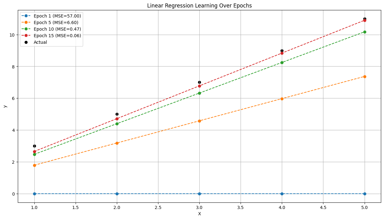
    if (i+1) % 5 == 0 or i == 0:
        plt.plot(X, y_pred, marker='o', linestyle='--', label=f'Epoch {i+1} (MSE={mse:.2f})')

# Plot actual data
plt.scatter(X, y, color='black', label='Actual')
plt.xlabel('X')
plt.ylabel('y')
plt.title('Linear Regression Learning Over Epochs')
plt.legend()
plt.grid(True)
plt.show()

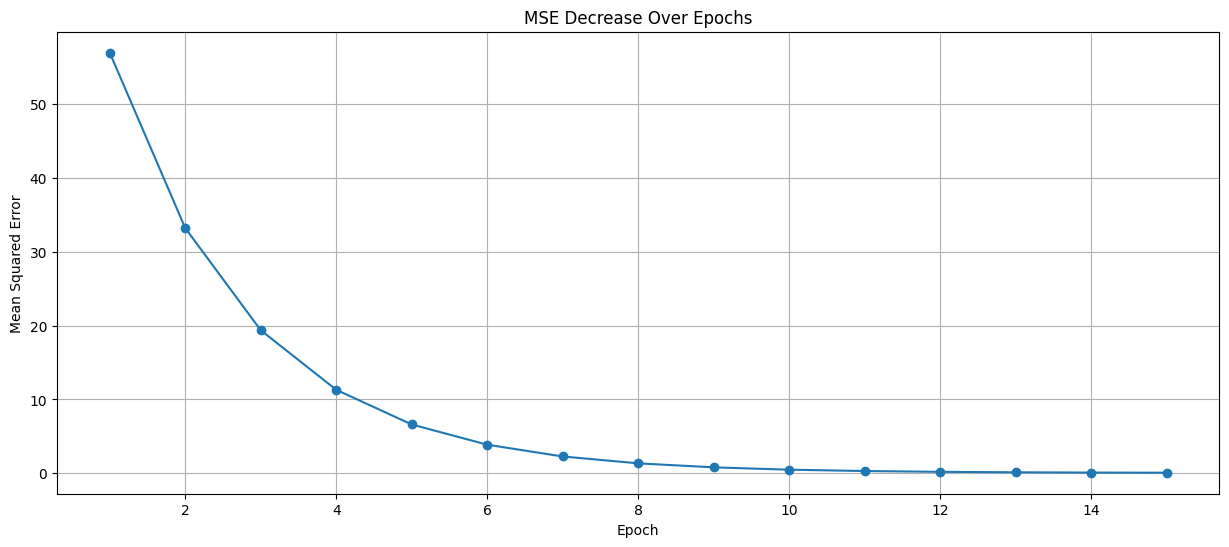
# Plot MSE over epochs
plt.figure(figsize=(15,6))
plt.plot(range(1, epochs+1), mse_list, marker='o', linestyle='-')
plt.xlabel('Epoch')
plt.ylabel('Mean Squared Error')
plt.title('MSE Decrease Over Epochs')
plt.grid(True)
plt.show()

Oputput:

Epoch |  Init W  |  Init B  |           Pred y               |    MSE     |   Grad W   |   Grad B   |  Upd W   |  Upd B  
------------------------------------------------------------------------------------------------------------------------
 |  0.0000  |  0.0000  | [0.00, 0.00, 0.00, 0.00, 0.00] |  57.0000   |  -50.0000  |  -14.0000  |  0.5000  |  0.1400 
 |  0.5000  |  0.1400  | [0.64, 1.14, 1.64, 2.14, 2.64] |  33.2296   |  -38.1600  |  -10.7200  |  0.8816  |  0.2472 
 |  0.8816  |  0.2472  | [1.13, 2.01, 2.89, 3.77, 4.66] |  19.3773   |  -29.1216  |  -8.2160   |  1.1728  |  0.3294 
 |  1.1728  |  0.3294  | [1.50, 2.67, 3.85, 5.02, 6.19] |  11.3048   |  -22.2219  |  -6.3044   |  1.3950  |  0.3924 
 |  1.3950  |  0.3924  | [1.79, 3.18, 4.58, 5.97, 7.37] |   6.6004   |  -16.9548  |  -4.8450   |  1.5646  |  0.4409 
 |  1.5646  |  0.4409  | [2.01, 3.57, 5.13, 6.70, 8.26] |   3.8589   |  -12.9341  |  -3.7308   |  1.6939  |  0.4782 
 |  1.6939  |  0.4782  | [2.17, 3.87, 5.56, 7.25, 8.95] |   2.2612   |  -9.8647   |  -2.8801   |  1.7926  |  0.5070 
 |  1.7926  |  0.5070  | [2.30, 4.09, 5.88, 7.68, 9.47] |   1.3300   |  -7.5217   |  -2.2307   |  1.8678  |  0.5293 
 |  1.8678  |  0.5293  | [2.40, 4.26, 6.13, 8.00, 9.87] |   0.7873   |  -5.7331   |  -1.7347   |  1.9251  |  0.5466 
 |  1.9251  |  0.5466  | [2.47, 4.40, 6.32, 8.25, 10.17] |   0.4709   |  -4.3677   |  -1.3561   |  1.9688  |  0.5602 
 |  1.9688  |  0.5602  | [2.53, 4.50, 6.47, 8.44, 10.40] |   0.2865   |  -3.3254   |  -1.0669   |  2.0020  |  0.5708 
 |  2.0020  |  0.5708  | [2.57, 4.57, 6.58, 8.58, 10.58] |   0.1789   |  -2.5298   |  -0.8460   |  2.0273  |  0.5793 
 |  2.0273  |  0.5793  | [2.61, 4.63, 6.66, 8.69, 10.72] |   0.1162   |  -1.9225   |  -0.6773   |  2.0466  |  0.5861 
 |  2.0466  |  0.5861  | [2.63, 4.68, 6.73, 8.77, 10.82] |   0.0795   |  -1.4589   |  -0.5484   |  2.0612  |  0.5916 
 |  2.0612  |  0.5916  | [2.65, 4.71, 6.78, 8.84, 10.90] |   0.0581   |  -1.1051   |  -0.4499   |  2.0722  |  0.5961 

Charts:
Linear Regression Learning Over Epochs

MSE Decrease Over Epochs