Demystifying K-Means Clustering
(A Complete Guide with Step-by-Step Mathematical and Python Code)
Welcome to a detailed exploration of K-Means Clustering, one of the most fundamental algorithms in data science. This blog post isn’t just a conceptual overview—it is a complete journey, starting from the basic definitions, walking through a mathematical example calculation step by step, showing how to implement it in Python, and finally, explaining how to measure success.
Whether you are a student, a beginner, or just need a solid refresh, this guide will make K-Means crystal clear.
1. Introduction to Clustering
Before we dive into the algorithm, let’s establish the context: unsupervised machine learning.
What is Clustering?
At its heart, Clustering is about finding groups within data. It is the process of grouping similar data points together while keeping dissimilar points separated.
It is a type of unsupervised learning, which means the algorithm works on unlabeled data. We don’t have a “right answer” (a label like “cat” or “dog”); the algorithm must discover the structure, patterns, and relationships within the data on its own.
Applications of Clustering
If you need to make sense of large amounts of diverse data without previous categories, clustering is your go-to tool. It is used in:
- Customer Segmentation: Businesses analyze purchasing behavior to group customers (e.g., “high spenders,” “occasional buyers”) for targeted marketing.
- Image Compression: By grouping pixels with similar colors together and using the group center as a single color, images can be compressed significantly.
- Anomaly Detection: By clustering standard patterns of data (like bank transactions or sensor readings), data points that fall far outside of any cluster can be identified as potential fraud or system errors.
2. What is K-Means?
The Core Concept
K-Means is a specific, popular partitioning-based clustering algorithm. Its objective is to divide a dataset into \(K\) distinct, non-overlapping subsets (clusters) based on the similarity of the data points.
The Objective Function
The main goal of K-Means can be summarized as:
- Minimize Intra-cluster distance: Make points inside the same cluster as close (similar) as possible to each other. This is measured by how close points are to their cluster center (centroid).
- Maximize Inter-cluster distance: Keep the clusters themselves as far away (dissimilar) as possible from each other.
3. How K-Means Works (Step-by-Step)
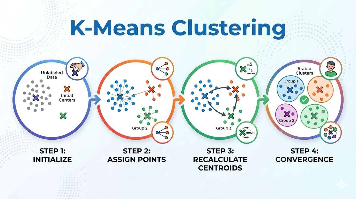
The beauty of K-Means lies in its simple, iterative process. Here is how it functions, step-by-step:
[Image: A diagram showing the iterative steps of K-Means Clustering]
Step 1: Choose K
The first and most critical decision is deciding the number of clusters, \(K\). We will discuss how to choose this optimally later.
Step 2: Initialize Centroids
K-Means starts by placing \(K\) points into the feature space. These initial points are called centroids (the centers of the clusters).
- They can be initialized randomly by picking \(K\) random data points from the dataset.
- Better methods exist, such as K-Means++, which initializes centroids far apart from each other, speeding up convergence and avoiding bad local optima.
Step 3: Assign Points
This is the optimization part. For every single data point in your entire dataset:
- Calculate its distance to all \(K\) centroids.
- Assign the point to the cluster of the nearest centroid.
A point is assigned to Cluster \(j\) if the distance to Centroid \(j\) is the minimum among all centroid distances.
Step 4: Recalculate Centroids
Now that points are assigned, each centroid must find the “true center” of its newly assigned members. The position of each centroid is updated by calculating the mean (average) of all data points that are currently members of that cluster.
If a cluster has points \(P_1, P_2, \dots, P_n\), the new centroid is: \(C_{new} = \left(\frac{1}{n} \sum P_{ix}, \frac{1}{n} \sum P_{iy}\right)\)
Step 5: Repeat Until Convergence
Steps 3 and 4 are repeated (iterated) until convergence. Convergence is reached when the centroids stop changing position (or change very little). At this point, the algorithm has stabilized, and the points are fixed in their best-guess clusters.
4. A Mathematical Example Step-by-Step
concept is good, but math makes it real. Let’s walk through the exact data provided in the example above.
We will use Euclidean Distance as our measure of similarity. For two points \((x_1, y_1)\) and \((x_2, y_2)\), the distance \(d\) is: \(d = \sqrt{(x_2 - x_1)^2 + (y_2 - y_1)^2}\)
Dataset and Initial Conditions
- Data Points: \(\{A1(2,10), A2(2,5), A3(8,4), B1(5,8), B2(7,5), B3(6,4), C1(1,2), C2(4,9)\}\)
- Initial Centroids: We choose \(K=3\) and start with specific (fixed) points:
- Centroid A: \((2, 10)\)
- Centroid B: \((5, 8)\)
- Centroid C: \((1, 2)\)
Iteration 1
We calculate the distance of all 8 points to these 3 initial centroids.
Table 1: Iteration 1 Distance Calculations and Assignments
| Point | x | y | dist to A (2,10) | dist to B (5,8) | dist to C (1,2) | Cluster Assignment |
|---|---|---|---|---|---|---|
| A1 | 2 | 10 | 0.000 | 3.606 | 8.062 | A |
| A2 | 2 | 5 | 5.000 | 4.243 | 3.162 | C (Moved!) |
| A3 | 8 | 4 | 8.485 | 5.000 | 7.280 | B |
| B1 | 5 | 8 | 3.606 | 0.000 | 7.211 | B |
| B2 | 7 | 5 | 7.071 | 3.606 | 6.708 | B |
| B3 | 6 | 4 | 7.211 | 4.123 | 5.385 | B |
| C1 | 1 | 2 | 8.062 | 7.211 | 0.000 | C |
| C2 | 4 | 9 | 2.236 | 1.414 | 7.616 | B (Moved!) |
Analysis of Iteration 1:
- Point A2 is closest to Centroid C (\(3.162\)), not A (\(5.000\)), so it joins Cluster C.
- Point C2 is closest to Centroid B (\(1.414\)), not C (\(7.616\)), so it joins Cluster B.
Recalculating New Centroids for Iteration 2
Since points moved, we must re-calculate the means of the new groupings:
- New Group A: \(\{A1\}\) -> Mean: (2, 10)
- New Group B: \(\{A3, B1, B2, B3, C2\}\)
- \[x = \frac{8+5+7+6+4}{5} = 6.0\]
- \[y = \frac{4+8+5+4+9}{5} = 6.0\]
- New Centroid B: (6, 6)
- New Group C: \(\{A2, C1\}\)
- \[x = \frac{2+1}{2} = 1.5\]
- \[y = \frac{5+2}{2} = 3.5\]
- New Centroid C: (1.5, 3.5)
Iteration 2
We use these updated centroids to recalculate all distances.
Table 2: Iteration 2 Distance Calculations and Assignments
| Point | x | y | dist to A (2,10) | dist to B (6,6) | dist to C (1.5,3.5) | Cluster Assignment |
|---|---|---|---|---|---|---|
| A1 | 2 | 10 | 0.000 | 5.657 | 6.519 | A |
| A2 | 2 | 5 | 5.000 | 4.123 | 1.581 | C |
| A3 | 8 | 4 | 8.485 | 2.828 | 6.519 | B |
| B1 | 5 | 8 | 3.606 | 2.236 | 5.701 | B |
| B2 | 7 | 5 | 7.071 | 1.414 | 5.701 | B |
| B3 | 6 | 4 | 7.211 | 2.000 | 4.528 | B |
| C1 | 1 | 2 | 8.062 | 6.403 | 1.581 | C |
| C2 | 4 | 9 | 2.236 | 3.606 | 6.042 | A (Moved!) |
Analysis of Iteration 2:
- C2 has shifted again! Centroid B moved far to the right (to \(x=6.0\)), and Centroid C moved slightly up. Point C2 \((4,9)\) is now much closer to Centroid A \((2,10)\) at \(2.236\) than to Centroid B \((3.606)\). It joins Cluster A.
Recalculating New Centroids for Iteration 3
- New Group A: \(\{A1, C2\}\) -> \(x=\frac{2+4}{2}=3.0\), \(y=\frac{10+9}{2}=9.5\) -> Centroid: (3.0, 9.5)
- New Group B: \(\{A3, B1, B2, B3\}\) -> \(x=\frac{8+5+7+6}{4}=6.5\), \(y=\frac{4+8+5+4}{4}=5.25\) -> Centroid: (6.5, 5.25)
- New Group C: \(\{A2, C1\}\) -> (1.5, 3.5) (unchanged)
Iteration 3
We perform the distance check one more time.
Table 3: Iteration 3 Distance Calculations and Assignments
| Point | x | y | dist to A (3,9.5) | dist to B (6.5,5.25) | dist to C (1.5,3.5) | Cluster Assignment |
|---|---|---|---|---|---|---|
| A1 | 2 | 10 | 1.118 | 6.543 | 6.519 | A |
| A2 | 2 | 5 | 4.610 | 4.507 | 1.581 | C |
| A3 | 8 | 4 | 7.433 | 1.953 | 6.519 | B |
| B1 | 5 | 8 | 2.500 | 3.132 | 5.701 | A (Moved!) |
| B2 | 7 | 5 | 6.021 | 0.559 | 5.701 | B |
| B3 | 6 | 4 | 6.265 | 1.346 | 4.528 | B |
| C1 | 1 | 2 | 7.762 | 6.388 | 1.581 | C |
| C2 | 4 | 9 | 1.118 | 4.507 | 6.042 | A |
Analysis of Iteration 3:
- Another shift! B1 \((5,8)\) was originally in Cluster B, but as the centroids shifted, it became significantly closer to the new Centroid A \((2.500)\) than to the new Centroid B \((3.132)\). It joins Cluster A.
Recalculating New Centroids for Iteration 4
- New Group A: \(\{A1, B1, C2\}\) -> \(x \approx 3.667\), \(y=9.0\) -> Centroid: (3.667, 9.0)
- New Group B: \(\{A3, B2, B3\}\) -> \(x=7.0\), \(y \approx 4.333\) -> Centroid: (7.0, 4.333)
- New Group C: \(\{A2, C1\}\) -> (1.5, 3.5) (unchanged)
Iteration 4 (Final Check)
Because we calculate new distances again for this step, but none of the cluster assignments change from Iteration 3. For example, B1 remains closest to Centroid A (\(1.667\)), not Centroid B (\(4.216\)).
Since the assignments (and thus the centroids) are exactly the same as the previous step, the algorithm is stable and converged.
Final Summary:
- Cluster A \(\{A1, B1, C2\}\) — Centroid (3.67, 9.00)
- Cluster B \(\{A3, B2, B3\}\) — Centroid (7.00, 4.33)
- Cluster C \(\{A2, C1\}\) — Centroid (1.50, 3.50)
This mathematical journey shows exactly how points move from initial fixed points to find their final clusters over 4 iterations.
5. K-Means Implementation from Scratch in Python
Now that you’ve done the math manually, let’s look at the implementation using Python. This code does exactly what we described above iterative.
import math
import pandas as pd

# 1. Define the Dataset
# We define our data points as a dictionary of coordinate tuples.
points_data = {
    'A1': (2, 10), 'A2': (2, 5), 'A3': (8, 4),
    'B1': (5, 8),  'B2': (7, 5), 'B3': (6, 4),
    'C1': (1, 2),  'C2': (4, 9)
}

# 2. Set Initial Centroids (Iteration 1)
# These are the same starting points we used in our math example.
initial_centroids = {
    'A': (2, 10),
    'B': (5, 8),
    'C': (1, 2)
}

def euclidean_distance(p1, p2):
    """Calculates the Euclidean distance between two points."""
    return math.sqrt((p1[0] - p2[0])**2 + (p1[1] - p2[1])**2)

def run_kmeans_with_tables(points, centroids, max_iterations=10):
    """Executes the K-Means algorithm and prints the state at each step."""
    current_centroids = centroids.copy()

    for i in range(max_iterations):
        print(f"\n--- ITERATION {i+1} ---")
        rows = []
        clusters = {name: [] for name in current_centroids}

        # --- Step 1: Cluster Assignment ---
        # For every point, calculate distance to current A, B, and C centers.
        for p_name, p_coords in points.items():
            dist_a = euclidean_distance(p_coords, current_centroids['A'])
            dist_b = euclidean_distance(p_coords, current_centroids['B'])
            dist_c = euclidean_distance(p_coords, current_centroids['C'])

            # Find the closest of the three
            dists = {'A': dist_a, 'B': dist_b, 'C': dist_c}
            assigned_cluster = min(dists, key=dists.get)

            # Record membership
            clusters[assigned_cluster].append(p_coords)

            # Prepare this information to display in our table
            rows.append({
                'Point': p_name,
                'x': p_coords[0],
                'y': p_coords[1],
                'dist to A': round(dist_a, 3),
                'dist to B': round(dist_b, 3),
                'dist to C': round(dist_c, 3),
                'Cluster': assigned_cluster
            })

        # --- Display the Table for this Iteration ---
        df = pd.DataFrame(rows)
        # Replicates the structure of the input slide/table.
        print(df.to_string(index=False))

        # --- Step 2: Calculate New Centroids ---
        new_centroids = {}
        print("\nRecalculating new centroids based on mean positions...")
        for c_name, members in clusters.items():
            if members:
                avg_x = sum(p[0] for p in members) / len(members)
                avg_y = sum(p[1] for p in members) / len(members)
                # Store new centroid, rounding for neat output
                new_centroids[c_name] = (round(avg_x, 3), round(avg_y, 3))
                print(f"Centroid {c_name} moved to: {new_centroids[c_name]}")
            else:
                # If a cluster became empty, keep the centroid where it was
                new_centroids[c_name] = current_centroids[c_name]

        # --- Step 3: Check for Convergence ---
        if new_centroids == current_centroids:
            print("\nConvergence reached! Assignments stop changing.")
            break

        # Prep for the next iteration
        current_centroids = new_centroids

# Run the entire process and view the math tables live!
run_kmeans_with_tables(points_data, initial_centroids)
Ouptput:
--- ITERATION 1 ---
Point  x  y  dist to A  dist to B  dist to C Cluster
   A1  2 10      0.000      3.606      8.062       A
   A2  2  5      5.000      4.243      3.162       C
   A3  8  4      8.485      5.000      7.280       B
   B1  5  8      3.606      0.000      7.211       B
   B2  7  5      7.071      3.606      6.708       B
   B3  6  4      7.211      4.123      5.385       B
   C1  1  2      8.062      7.211      0.000       C
   C2  4  9      2.236      1.414      7.616       B

Recalculating new centroids based on mean positions...
Centroid A moved to: (2.0, 10.0)
Centroid B moved to: (6.0, 6.0)
Centroid C moved to: (1.5, 3.5)

--- ITERATION 2 ---
Point  x  y  dist to A  dist to B  dist to C Cluster
   A1  2 10      0.000      5.657      6.519       A
   A2  2  5      5.000      4.123      1.581       C
   A3  8  4      8.485      2.828      6.519       B
   B1  5  8      3.606      2.236      5.701       B
   B2  7  5      7.071      1.414      5.701       B
   B3  6  4      7.211      2.000      4.528       B
   C1  1  2      8.062      6.403      1.581       C
   C2  4  9      2.236      3.606      6.042       A

Recalculating new centroids based on mean positions...
Centroid A moved to: (3.0, 9.5)
Centroid B moved to: (6.5, 5.25)
Centroid C moved to: (1.5, 3.5)

--- ITERATION 3 ---
Point  x  y  dist to A  dist to B  dist to C Cluster
   A1  2 10      1.118      6.543      6.519       A
   A2  2  5      4.610      4.507      1.581       C
   A3  8  4      7.433      1.953      6.519       B
   B1  5  8      2.500      3.132      5.701       A
   B2  7  5      6.021      0.559      5.701       B
   B3  6  4      6.265      1.346      4.528       B
   C1  1  2      7.762      6.388      1.581       C
   C2  4  9      1.118      4.507      6.042       A

Recalculating new centroids based on mean positions...
Centroid A moved to: (3.667, 9.0)
Centroid B moved to: (7.0, 4.333)
Centroid C moved to: (1.5, 3.5)

--- ITERATION 4 ---
Point  x  y  dist to A  dist to B  dist to C Cluster
   A1  2 10      1.944      7.557      6.519       A
   A2  2  5      4.333      5.044      1.581       C
   A3  8  4      6.616      1.054      6.519       B
   B1  5  8      1.666      4.177      5.701       A
   B2  7  5      5.207      0.667      5.701       B
   B3  6  4      5.518      1.054      4.528       B
   C1  1  2      7.491      6.438      1.581       C
   C2  4  9      0.333      5.548      6.042       A

Recalculating new centroids based on mean positions...
Centroid A moved to: (3.667, 9.0)
Centroid B moved to: (7.0, 4.333)
Centroid C moved to: (1.5, 3.5)

Convergence reached! Assignments stop changing.
6. Metrics and Choosing the Right K
In the previous sections, we walked through the mechanics of K-Means using a small dataset. But in the real world, data doesn’t come with labels, and it certainly doesn’t come with a manual telling you how many clusters exist. How do we know if our model is actually “good”? To answer this, we look at WCSS and the Silhouette Score.
Choosing the Right K: The Elbow Method
The most common question in clustering is: “How many clusters (\(K\)) should I use?” To solve this, we track the Within-Cluster Sum of Squares (WCSS). This metric calculates the sum of the squared distances between each data point and its assigned cluster centroid. Mathematically, it looks like this:
\[WCSS = \sum_{i=1}^{K} \sum_{P \in Cluster_i} \text{dist}(P, Centroid_i)^2\]The Logic:
- We want WCSS to be low, as a low value means points are very close to their centers (high density).
- However, as \(K\) increases, WCSS naturally drops. If we have \(10\) points and set \(K=10\), WCSS becomes \(0\) because every point is its own centroid. This isn’t helpful—it’s overfitting.
The “Sweet Spot” Example
Think of the Elbow Method like a cost-benefit analysis. When you plot WCSS against \(K\), the graph typically looks like an arm.
- The Drop: From \(K=1\) to \(K=3\), you usually see a massive drop in WCSS. This indicates that adding these clusters is significantly improving the model.
- The Elbow: At a certain point (e.g., \(K=4\)), the rate of decrease slows down significantly. The graph “bends.”
- Diminishing Returns: Past the elbow, adding more clusters only reduces WCSS by a tiny amount, but increases the complexity of your model. We choose the \(K\) value at the elbow.
Silhouette Score: A Sophisticated Metric
While the Elbow Method tells us about the “tightness” of clusters, the Silhouette Score tells us about their separation. It asks: “Is this point closer to its own group than to the next nearest group?”
For any given point \(i\), we calculate two values:
- Cohesion (\(a(i)\)): The average distance between point \(i\) and all other points in the same cluster. We want this to be small.
- Separation (\(b(i)\)): The average distance between point \(i\) and all points in the nearest neighboring cluster. We want this to be large.
The Silhouette Coefficient \(s(i)\) is then: \(s(i) = \frac{b(i) - a(i)}{\max(a(i), b(i))}\)
Interpreting the Score
The score ranges from -1 to +1:
- Near +1: The point is far away from neighboring clusters and right in the middle of its own. This is the goal!
- Near 0: The point is on the boundary between two clusters.
- Near -1: The point is likely in the wrong cluster.
Why use this over the Elbow Method? The Elbow Method only looks at how tight the clusters are. The Silhouette Score is more “sophisticated” because it validates if the clusters are distinct enough from one another. If your average Silhouette Score is low, it’s a sign that your clusters are overlapping too much, regardless of what the Elbow plot says.
Final Thoughts
K-Means Clustering is a cornerstone of unsupervised learning. It allows us to uncover hidden structures in data without needing prior labels. Through our journey, we’ve covered:
- The Mechanism: How centroids “pull” points toward them and shift based on the mean.
- The Math: Using Euclidean distance to drive assignments.
- The Code: Implementing the logic from scratch to understand the “brain” of the algorithm.
- The Metrics: Using the Elbow Method and Silhouette Score to ensure we aren’t just grouping data for the sake of it, but finding meaningful, distinct patterns.
You are now equipped with both the theoretical “why” and the technical “how” of K-Means. Whether you are segmenting customers or organizing image pixels, the principles remain the same: minimize the distance within, maximize the distance between.