Standard Deviation — Statistics & NumPy
(Measuring the Spread of Data)
1. Introduction
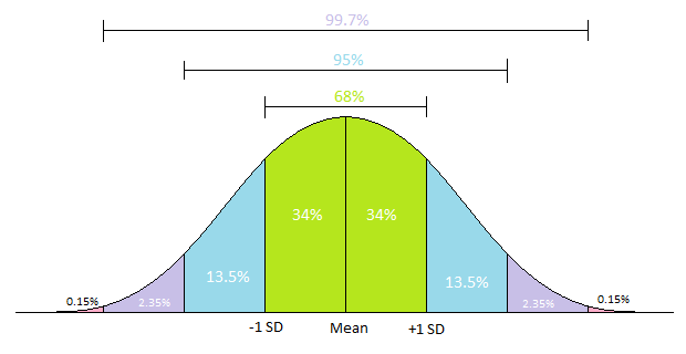
The Standard Deviation (SD) is one of the most important measures in statistics. While the mean tells us the central value of a dataset, the standard deviation tells us how much the data points deviate from that mean.
In other words, it measures the spread or dispersion of data. A low standard deviation means the data points are close to the mean, while a high standard deviation means they are more spread out.
2. Mathematical Concept
Step-by-Step Intuition
Let’s say we have a dataset:
\[X = [2, 4, 6, 8, 10]\]-
Find the mean (\(\bar{X}\))
\[\bar{X} = \frac{2 + 4 + 6 + 8 + 10}{5} = 6\] -
Find each deviation from the mean
\[(x_i - \bar{X}) = [-4, -2, 0, 2, 4]\] -
Square each deviation
\[(x_i - \bar{X})^2 = [16, 4, 0, 4, 16]\] -
Find the average of squared deviations
This is the Variance (\(\sigma^2\)):
\[\sigma^2 = \frac{16 + 4 + 0 + 4 + 16}{5} = 8\] -
Take the square root of the variance
This gives the Standard Deviation (\(\sigma\)):
\[\sigma = \sqrt{8} = 2.828\]
3. Formula
For a population (complete data):
\[\sigma = \sqrt{\frac{1}{N}\sum_{i=1}^{N}(x_i - \bar{x})^2}\]For a sample (subset of data):
\[s = \sqrt{\frac{1}{N-1}\sum_{i=1}^{N}(x_i - \bar{x})^2}\]The denominator difference (
NvsN-1) adjusts for bias when estimating from a sample.
4. Relationship with Variance
Variance and Standard Deviation are closely related:
\[\sigma^2 = \text{Variance}, \quad \sigma = \sqrt{\text{Variance}}\]So the standard deviation is simply the square root of variance.
5. Interpretation
- Small SD (≈0) → data points are close to the mean (less spread).
- Large SD → data points are far from the mean (more spread).
- SD = 0 → all values are identical.
For example:
- Test scores with a low SD mean students performed similarly.
- A high SD means some scored much higher/lower than average.
6. Using NumPy: np.std() and np.var()
NumPy makes it easy to compute both variance and standard deviation.
Example 1:
import numpy as np

data = np.array([2, 4, 6, 8, 10])

# Standard Deviation
std_population = np.std(data)
std_sample = np.std(data, ddof=1)  # sample SD

# Variance (for reference)
var_population = np.var(data)
var_sample = np.var(data, ddof=1)

print("Population Standard Deviation:", std_population)
print("Sample Standard Deviation:", std_sample)
print("Population Variance:", var_population)
print("Sample Variance:", var_sample)
Output:
Population Standard Deviation: 2.8284271247461903
Sample Standard Deviation: 3.1622776601683795
Population Variance: 8.0
Sample Variance: 10.0
7. Real-Life Analogy
Imagine you and four friends run 100m sprints:
| Person | Time (seconds) |
|---|---|
| A | 12 |
| B | 12 |
| C | 12 |
| D | 12 |
| E | 12 |
Mean = 12, Standard Deviation = 0
→ Everyone ran equally fast.
Now suppose the times are [10, 11, 12, 13, 14].
Mean = 12, SD = 1.41
→ The performances varied around the mean.
8. Key Takeaways
| Concept | Symbol | Formula | Description |
|---|---|---|---|
| Variance | \(\sigma^2\) | \(\frac{1}{N}\sum(x_i - \bar{x})^2\) | Average of squared deviations |
| Standard Deviation | \(\sigma\) | \(\sqrt{\sigma^2}\) | Root of variance — shows spread |
| Population SD | — | divide by N |
Entire data |
| Sample SD | — | divide by N-1 |
Subset data |
9. Summary
- Standard deviation measures how spread out your data is.
- It’s always non-negative.
- Useful in finance (volatility), science (measurement accuracy), ML (feature scaling), and more.
- In NumPy,
np.std()andnp.var()provide fast, vectorized computation.